Universal approximators#
In this section, we’ll look at various ways to fit a non-linear function without knowing its functional form, which will lead us to a simple neural network.
Sample problem#
Suppose you’re trying to fit this crazy function:
import numpy as np
import matplotlib.pyplot as plt
def truth(x):
    return np.where(abs(x - 0.43) < 0.15, np.sin(22*x), -1 + 3.5*x - 2*x**2)

x = np.random.uniform(0, 1, 1000)
y = truth(x) + np.random.normal(0, 0.03, 1000)
fig, ax = plt.subplots()

curve_x = np.linspace(0, 1, 1000)
curve_y = truth(curve_x)

ax.scatter(x, y, marker=".", label="data to fit")
ax.plot(curve_x, curve_y, color="magenta", linewidth=3, label="truth")

ax.legend(loc="lower right")

plt.show()
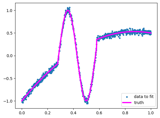
I don’t think I need to demonstrate that a linear fit would be terrible.
We can get a good fit from a theory-driven ansatz, but as I showed in the previous section, it’s very sensitive to the initial guess that we give the fitter.
What’s next?
Taylor series#
As a physicist, “Taylor series” might have been your first thought!
Taylor series are used heavily throughout theoretical and experimental physics, as a formally correct infinite series, as a one-term approximation, and everything in between. Even \(E = mc^2\) is the first term of a Taylor series:
where the second term is classical kinetic energy.
A Taylor (or Maclaurin) series is a decomposition of a function into infinitely many pieces:
where each \(a_n\) is computed from the \(n\)th derivative of the function, evaluated at zero.
The function \(f\) can be thought of as a single infinite-dimensional vector and we’re describing its components with all the \(a_n\). Any data with an analytic functional relationship between \(x\) and \(y\) can be expressed by an infinite set of fit parameters \(a_n\), though in practice, we’ll have to pick a finite set of parameters to approximate the shape. Since finitely many data points \(x_i\), \(y_i\) can’t tell us about infinitely many parameters anyway, this is fine.
Even better, these parameters can be determined as a solution to a system of linear equations, rather than an iterative search. On specific domains, Taylor coefficients are linearly related to coefficients of orthogonal polynomial series, such as Jacobi polynomials, Laguerre polynomials, Hermite polynomials, Chebyshev polynomials, etc. Every coefficient of an orthogonal expansion can be determined independently of every other, since they’re determined from integrals in which the integral of two basis functions is zero. Taylor series don’t exactly have this property, but since they’re only a linear transformation away, the Taylor coefficients can be computed in one step as an exact formula.
So while you could pass something like \(a_0 + a_1 x + a_2 x^2 + a_3 x^3\) as an ansatz to Minuit and run its iterative algorithm, you could instead get an exact best-fit without the possibility of fit-failure by using a linear algebra library. NumPy has a polynomial fitter built in, so let’s see the result.
NUMBER_OF_POLYNOMIAL_TERMS = 15

coefficients = np.polyfit(x, y, NUMBER_OF_POLYNOMIAL_TERMS - 1)[::-1]

model_x = np.linspace(0, 1, 1000)
model_y = sum(c * model_x**i for i, c in enumerate(coefficients))
fig, ax = plt.subplots()

ax.scatter(x, y, marker=".")
ax.plot(curve_x, curve_y, color="magenta", linewidth=3)
ax.plot(model_x, model_y, color="orange", linewidth=3)

ax.legend(["measurements", "truth", f"{len(coefficients)} Taylor components"], loc="lower right")

plt.show()
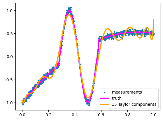
It’s kind of wiggily. It’s a relatively good fit on the big oscillation, since that part looks like a polynomial, but it can’t dampen the oscillations on the flat parts without a lot more terms.
Increasing the number of terms makes it look better:
NUMBER_OF_POLYNOMIAL_TERMS = 100

coefficients = np.polyfit(x, y, NUMBER_OF_POLYNOMIAL_TERMS - 1)[::-1]

model_x = np.linspace(0, 1, 1000)
model_y = sum(c * model_x**i for i, c in enumerate(coefficients))
/tmp/ipykernel_2209/1978071889.py:3: RankWarning: Polyfit may be poorly conditioned
  coefficients = np.polyfit(x, y, NUMBER_OF_POLYNOMIAL_TERMS - 1)[::-1]
fig, ax = plt.subplots()

ax.scatter(x, y, marker=".")
ax.plot(curve_x, curve_y, color="magenta", linewidth=3)
ax.plot(model_x, model_y, color="orange", linewidth=3)

ax.legend(["measurements", "truth", f"{len(coefficients)} Taylor components"], loc="lower right")

plt.show()
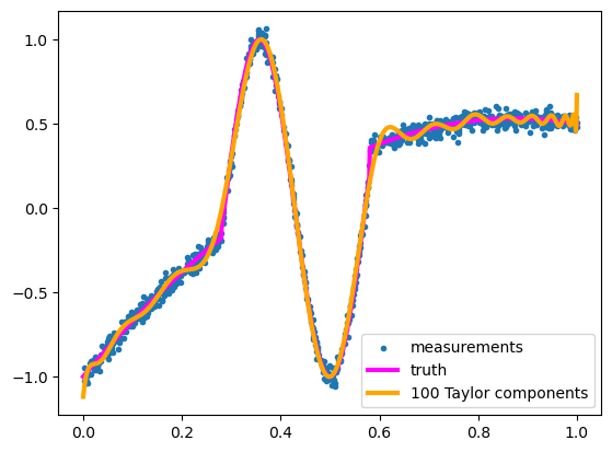
But not outside the domain of \(x\) values that it was fitted to.
fig, ax = plt.subplots()

model_x_2 = np.linspace(0, 2, 2000)
model_y_2 = sum(c * model_x_2**i for i, c in enumerate(coefficients))

curve_x_2 = np.linspace(0, 2, 2000)
curve_y_2 = truth(curve_x_2)

ax.scatter(x, y, marker=".")
ax.plot(curve_x_2, curve_y_2, color="magenta", linewidth=3)
ax.plot(model_x_2, model_y_2, color="orange", linewidth=3)

ax.legend(["measurements", "truth", f"{len(coefficients)} Taylor components"], loc="upper right")
ax.set_ylim(-1.5, 2.5)

plt.show()
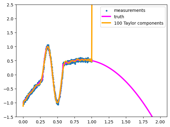
If our only knowledge of the function comes from its sampled points, there isn’t a “correct answer” for what the function should be outside of the sampled domain, but it probably shouldn’t shoot off into outer space.
This is a failure to generalize—we want our function approximation to make reasonable predictions outside of its training data. What “reasonable” means depends on the application, but if these were measurements of quantities in nature, unmeasured values at \(x > 1\) would probably be about \(2 < y < 2\).
Fourier series#
Your next thought, as a physicist, might be “Fourier series.”
Fourier series are also heavily used throughout physics. For instance, did you know that epicycles in medieval astronomy are the first few terms in a Fourier series? Discrete Fourier series approximate periodic functions and integral Fourier transforms approximate non-periodic functions. Like Taylor series, Fourier series are a decomposition of a function as an infinite-dimensional vector into infinitely many components, and Fourier components are orthogonal to each other. Instead of polynomial basis vectors, Fourier basis vectors are sine and cosine functions:
for some period \(P\). The coefficients are computed with integrals:
NumPy has a function for computing integrals using the trapezoidal rule, which I’ll use below to fit a Fourier series to the function.
NUMBER_OF_COS_TERMS = 7
NUMBER_OF_SIN_TERMS = 7

sort_index = np.argsort(x)
x_sorted = x[sort_index]
y_sorted = y[sort_index]

constant_term = np.trapz(y_sorted, x_sorted)
cos_terms = [2*np.trapz(y_sorted * np.cos(2*np.pi * (i + 1) * x_sorted), x_sorted) for i in range(NUMBER_OF_COS_TERMS)]
sin_terms = [2*np.trapz(y_sorted * np.sin(2*np.pi * (i + 1) * x_sorted), x_sorted) for i in range(NUMBER_OF_SIN_TERMS)]

model_x = np.linspace(0, 1, 1000)
model_y = (
    constant_term +
    sum(coefficient * np.cos(2*np.pi * (i + 1) * model_x) for i, coefficient in enumerate(cos_terms)) +
    sum(coefficient * np.sin(2*np.pi * (i + 1) * model_x) for i, coefficient in enumerate(sin_terms))
)
/tmp/ipykernel_2209/634007716.py:8: DeprecationWarning: `trapz` is deprecated. Use `trapezoid` instead, or one of the numerical integration functions in `scipy.integrate`.
  constant_term = np.trapz(y_sorted, x_sorted)
/tmp/ipykernel_2209/634007716.py:9: DeprecationWarning: `trapz` is deprecated. Use `trapezoid` instead, or one of the numerical integration functions in `scipy.integrate`.
  cos_terms = [2*np.trapz(y_sorted * np.cos(2*np.pi * (i + 1) * x_sorted), x_sorted) for i in range(NUMBER_OF_COS_TERMS)]
/tmp/ipykernel_2209/634007716.py:10: DeprecationWarning: `trapz` is deprecated. Use `trapezoid` instead, or one of the numerical integration functions in `scipy.integrate`.
  sin_terms = [2*np.trapz(y_sorted * np.sin(2*np.pi * (i + 1) * x_sorted), x_sorted) for i in range(NUMBER_OF_SIN_TERMS)]
fig, ax = plt.subplots()

ax.scatter(x, y, marker=".")
ax.plot(curve_x, curve_y, color="magenta", linewidth=3)
ax.plot(model_x, model_y, color="orange", linewidth=3)

ax.legend(["measurements", "truth", f"{1 + len(cos_terms) + len(sin_terms)} Fourier components"])

plt.show()
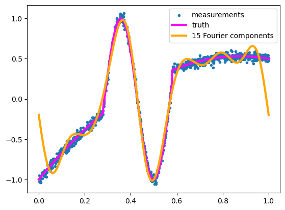
Like the Taylor series, this gets the large feature right and misses the edges. In fact, the Fourier model above is constrained to match at \(f(0) = f(1)\) because this is a discrete Fourier series and therefore periodic in the training domain.
Both the 15-term Taylor series and the 15-term Fourier series are not good fits to the function. In part, this is because the function is neither polynomial nor trigonometric, but a stitched-together monstrosity of both.
Adaptive basis functions#
The classic methods of universal function approximation—Taylor series, Fourier series, and others—have one thing in common: they all approximate the function with a fixed set of basis functions \(\psi_i\) for \(i \in [0, N)\).
Thus, you’re only allowed to optimize the coefficients \(c_i\) in front of each basis function, not the shapes of the basis functions themselves. You’re allowed to stack them, but not change them.
Suppose, instead, that we had a set of functions that could also change shape:
These are functions of \(x\), parameterized by \(\alpha_i\) and \(\beta_i\). Here’s an example set that we can use: sigmoid functions with an adjustable center \(\alpha\) and width \(\beta\):
def sigmoid_component(x, center, width):
    # ignore NumPy errors when Minuit explores extreme values
    with np.errstate(over="ignore", divide="ignore"):
        return 1 / (1 + np.exp((x - center) / width))
fig, ax = plt.subplots()

sample_x = np.linspace(0, 1, 1000)

ax.plot(model_x, sigmoid_component(sample_x, 0.5, 0.2), label=r"$\alpha = 0.5$, $\beta = 0.2$")
ax.plot(model_x, sigmoid_component(sample_x, 0.5, 0.1), label=r"$\alpha = 0.5$, $\beta = 0.1$")
ax.plot(model_x, sigmoid_component(sample_x, 0.75, -0.01), label=r"$\alpha = 0.75$, $\beta = -0.01$")

ax.legend(loc="lower left", bbox_to_anchor=(0.05, 0.1))

plt.show()
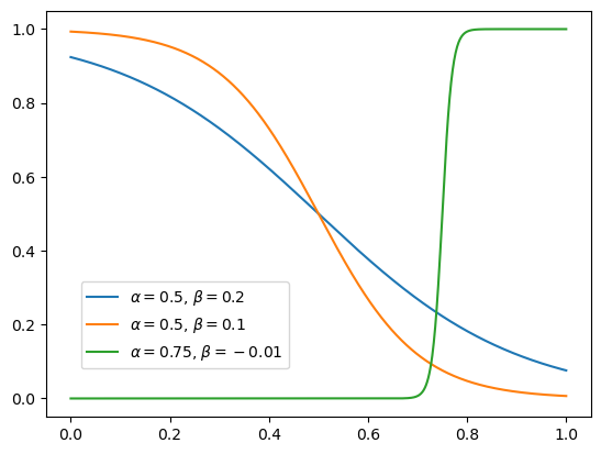
Fitting with these adaptive sigmoids requires an iterative search, rather than computing the parameters with an exact formula. These basis functions are not orthogonal to each other (unlike Fourier components), and they’re not even related through a linear transformation (unlike Taylor components).
In fact, this is a harder-than-usual problem for Minuit because the search space has many local minima. To get around this, let’s run it 15 times and take the best result (minimum of minima).
from iminuit import Minuit
from iminuit.cost import LeastSquares
NUMBER_OF_SIGMOIDS = 5

def sigmoid_sum(x, parameters):
    out = np.zeros_like(x)
    for coefficient, center, width in parameters.reshape(-1, 3):
        out += coefficient * sigmoid_component(x, center, width)
    return out

# using Minuit
least_squares = LeastSquares(x, y, 0.03, sigmoid_sum)

# do best of 15 optimizations
best_minimizer = None
for iteration in range(15):

    initial_parameters = np.zeros(5 * 3)
    initial_parameters[0::3] = np.random.normal(0, 1, NUMBER_OF_SIGMOIDS)    # coefficient terms
    initial_parameters[1::3] = np.random.uniform(0, 1, NUMBER_OF_SIGMOIDS)   # center parameters (alpha)
    initial_parameters[2::3] = np.random.normal(0, 0.1, NUMBER_OF_SIGMOIDS)  # width parameters (beta)

    minimizer = Minuit(least_squares, initial_parameters)
    minimizer.migrad()

    if best_minimizer is None or minimizer.fval < best_minimizer.fval:
        best_minimizer = minimizer

model_x = np.linspace(0, 1, 1000)
model_y = sigmoid_sum(model_x, np.array(best_minimizer.values))
fig, ax = plt.subplots()

ax.scatter(x, y, marker=".")
ax.plot(curve_x, curve_y, color="magenta", linewidth=3)
ax.plot(model_x, model_y, color="orange", linewidth=3)

ax.legend(["measurements", "truth", f"{len(minimizer.parameters)} sigmoid parameters"])

plt.show()
assert np.sum((model_y - curve_y)**2) < 10
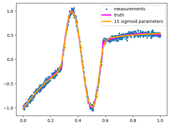
It’s a beautiful fit (usually)!
Since you used 5 sigmoids with 3 parameters each (scaling coefficient \(c_i\), center \(\alpha_i\), and width \(\beta_i\)), this is 15 parameters, and the result is much better than it is with 15 Taylor components or 15 Fourier components.
Moreover, it generalizes reasonably well:
fig, ax = plt.subplots()

model_x_2 = np.linspace(0, 2, 2000)
model_y_2 = sigmoid_sum(model_x_2, np.array(best_minimizer.values))

ax.scatter(x, y, marker=".")
ax.plot(curve_x_2, curve_y_2, color="magenta", linewidth=3)
ax.plot(model_x_2, model_y_2, color="orange", linewidth=3)

ax.legend(["measurements", "truth", f"{len(minimizer.parameters)} sigmoid parameters"])
ax.set_ylim(-1.5, 1.5)

plt.show()
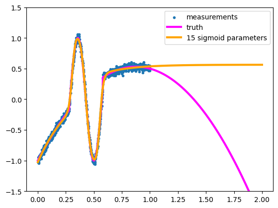
We can’t expect the fit to know what the true function does outside of the sample points, but it doesn’t shoot off into outer space or connect into a periodic function like Taylor or Fourier series do. It assumes that the curve levels off because it’s made out of components that level off.
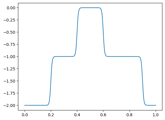
By varying the scale (\(c_i\)), center (\(\alpha_i\)), and width (\(\beta_i\)) of each sigmoid, we can build any sandcastle we want, and they all level off to horizontal lines outside the domain.
fig, ax = plt.subplots()

model_x = np.linspace(0, 1, 1000)

wide_plateau_left = sigmoid_component(model_x, 0.2, 0.005)
wide_plateau_right = sigmoid_component(model_x, 0.9, -0.005)

narrow_peak_left = sigmoid_component(model_x, 0.4, 0.005)
narrow_peak_right = sigmoid_component(model_x, 0.6, -0.005)

ax.plot(model_x, -wide_plateau_left - wide_plateau_right - narrow_peak_left - narrow_peak_right)

plt.show()
Adaptive basis functions are a one-layer neural network#
It may not look like it, but we’ve just crossed the (conventional) boundary from basic fitting to neural networks. The fit function
can be written as a linear-transformed \(x\) passed into a hard-coded sigmoid. Calling the hard-coded sigmoid \(f\):
and the linear-transformed \(x\) as \(x'_i\):
the full fit function is
We took a 1-dimensional \(x\), linear transformed it into an n-dimensional \(\vec{x}'\), applied a non-linear function \(f\), and then linear-transformed that into a 1-dimensional \(y\). Let’s draw it (for \(n = 5\)) like this:
If you’ve seen diagrams of neural networks before, this should look familiar! The input is on the left is a vertical column of boxes—only one in this case because our input is 1-dimensional—and the linear transformation is represented by arrows to the next vertical column of boxes, our 5-dimensional \(\vec{x}'\). The sigmoid \(f\) is not shown in diagram, and the next set of arrows represent another linear transformation to the outputs, \(y\), which is also 1-dimensional so only one box.
The first linear transform has slopes \(1/\beta\) and intercepts \(\alpha_i/\beta_i\) and the second linear transformation in our example has only slopes \(c_i\), but we could have added another intercept \(y_0\) if we wanted to, to let the vertical offset float.
In neural network terminology, the intermediate \(\vec{x}_i\) vector is a “hidden layer” between \(x\) and \(y\). The non-linear function applied at that layer is an “activation function.” Generally speaking (if you have enough parameters), the exact shape of the activation function isn’t important, but it cannot be linear, or else the two linear transformations would coalesce into one linear transformation. The activation function breaks the linearity that would make the \(c_i\) degenerate with the \(\alpha_i\) and \(\beta_i\) in the fit.
Conclusion#
We started with a generic regression problem: we wanted to fit a non-linear relationship between \(x_i\), \(y_i\) points without knowing the underlying functional form. A neural network with one hidden layer does the job because it’s really a collection of adaptive basis functions—like the classic Taylor and Fourier series, but more flexible and less extreme beyond the training domain. The fact that a single hidden layer can fit any functional form is called the Universal Approximation Theorem(s), but the mere fact that any shape can be approximated with sufficiently many terms is not as interesting as how it generalizes, particularly as you add more layers. After all, Taylor and Fourier series can approximate arbitrary functions, too.
In the next section, we’ll look at fully connected neural networks in general, and see what happens when you add more layers.
