Under and overfitting

import numpy as np
import matplotlib.pyplot as plt
from sklearn.linear_model import LinearRegression

In regression

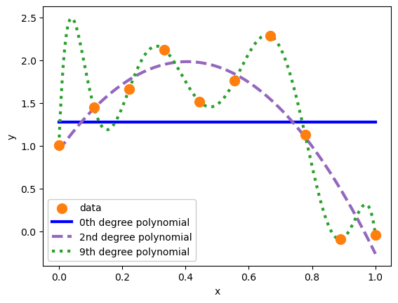
What do you think of these three fits?

data_x = np.linspace(0, 1, 10)
data_y = 1 + 4*data_x - 5*data_x**2 + np.random.normal(0, 0.3, 10)

def fit_polynomial(n):
    polynomial_features = np.hstack([data_x[:, np.newaxis]**i for i in range(n + 1)])
    best_fit = LinearRegression(fit_intercept=False).fit(polynomial_features, data_y)

    model_x = np.linspace(0, 1, 1000)
    polynomial_features = np.hstack([model_x[:, np.newaxis]**i for i in range(n + 1)])
    return model_x, best_fit.predict(polynomial_features)

fig, ax = plt.subplots()

ax.scatter(data_x, data_y, s=100, color="tab:orange", label="data", zorder=5)
ax.plot(*fit_polynomial(0), color="blue", linewidth=3, ls="-", label="0th degree polynomial")
ax.plot(*fit_polynomial(2), color="tab:purple", linewidth=3, ls="--", label="2nd degree polynomial")
ax.plot(*fit_polynomial(9), color="tab:green", linewidth=3, ls=":", label="9th degree polynomial")

ax.set_xlabel("x")
ax.set_ylabel("y")
ax.legend(loc="lower left", framealpha=1)

plt.show()

The first, a 0^th degree polynomial, is just an average. An average is the simplest model that has any relationship to the training data, but it’s usually too simple: it doesn’t characterize any functional relationships between features and targets and its predictions are sometimes far from the targets. This model underfits the data.

The second, a 2^nd degree polynomial, is just right for this data because it was generated from a 2^nd degree polynomial (\(1 + 4x - 5x^2\)).

The third, a 9^th degree polynomial, has more detail than the dataset itself. It makes false claims about what data would do between the points and beyond the domain. It overfits the data.

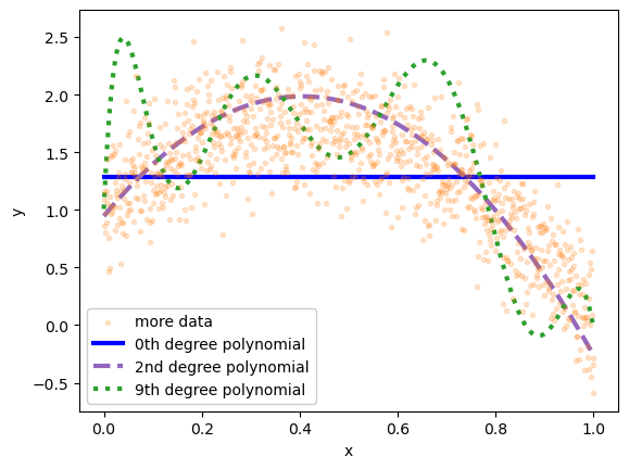
To see this, let’s overlay these models on a larger dataset with the same distribution.

more_data_x = np.linspace(0, 1, 1000)
more_data_y = 1 + 4*more_data_x - 5*more_data_x**2 + np.random.normal(0, 0.3, 1000)

fig, ax = plt.subplots()

ax.scatter(more_data_x, more_data_y, marker=".", color="tab:orange", alpha=0.20, label="more data", zorder=5)
ax.plot(*fit_polynomial(0), color="blue", linewidth=3, ls="-", label="0th degree polynomial")
ax.plot(*fit_polynomial(2), color="tab:purple", linewidth=3, ls="--", label="2nd degree polynomial")
ax.plot(*fit_polynomial(9), color="tab:green", linewidth=3, ls=":", label="9th degree polynomial")

ax.set_xlabel("x")
ax.set_ylabel("y")
ax.legend(loc="lower left", framealpha=1)

plt.show()

Although many of these new points are about 0.3 units from the 2^nd degree polynomial in \(y\), we can’t expect any better than that because that’s the precision, errors due to inherent randomness of the data. The 2^nd degree polynomial has high accuracy: the model is very close to the average \(y\) in small slices of \(x\).

The underfit 0^th degree polynomial is not accurate: in some regions of \(x\), the average \(y\) is far from its prediction. We could also say that the model is biased in some regions of \(x\). The random fluctuations are not centered on the model.

The overfit 9^th degree polynomial is not accurate either. But in this case, it’s because the model is too wiggly, trying to pass through the exact centers of the training data points, an exactness that is irrelevant to new samples of data drawn from the same distribution.

In classification

Let’s use penguin classification as an example.

import pandas as pd
import torch
from torch import nn, optim

penguins_df = pd.read_csv("data/penguins.csv")

categorical_int_df = penguins_df.dropna()[["bill_length_mm", "bill_depth_mm", "species"]]
categorical_int_df["species"], code_to_name = pd.factorize(categorical_int_df["species"].values)

feats = ["bill_length_mm", "bill_depth_mm"]
categorical_int_df[feats] = (
    categorical_int_df[feats] - categorical_int_df[feats].mean()
) / categorical_int_df[feats].std()

features = torch.tensor(categorical_int_df[feats].values, dtype=torch.float32)
targets = torch.tensor(categorical_int_df["species"].values, dtype=torch.int64)

Remember that a linear (logistic) fit to this dataset is sufficient:

model_without_softmax = nn.Sequential(
    nn.Linear(2, 3)
)

would be enough. But instead, we’re going to add 2 hidden layers with 10 vector components each.

model_without_softmax = nn.Sequential(
    nn.Linear(2, 10),     # 2 input features → 10 hidden on layer 1
    nn.ReLU(),
    nn.Linear(10, 10),    # 10 → 10 hidden on layer 2
    nn.ReLU(),
    nn.Linear(10, 3),     # 10 → 3 output categories
)

model_with_softmax = nn.Sequential(
    model_without_softmax,
    nn.Softmax(dim=1),
)

loss_function = nn.CrossEntropyLoss()

optimizer = optim.Adam(model_without_softmax.parameters())

for epoch in range(10000):
    optimizer.zero_grad()

    predictions = model_without_softmax(features)
    loss = loss_function(predictions, targets)

    loss.backward()
    optimizer.step()

fig, ax = plt.subplots(figsize=(6, 6))

background_x, background_y = np.meshgrid(np.linspace(-2.5, 2.5, 100), np.linspace(-2.5, 2.5, 100))
background_2d = np.column_stack([background_x.ravel(), background_y.ravel()])
probabilities = model_with_softmax(torch.tensor(background_2d, dtype=torch.float32)).detach().numpy()

for t in range(3):
    ax.contour(
        background_x, background_y, probabilities[:, t].reshape(background_x.shape), [0.5]
    )

    ax.scatter(
        categorical_int_df[feats].values[targets == t, 0],
        categorical_int_df[feats].values[targets == t, 1],
    )

ax.set_xlim(-2.5, 2.5)
ax.set_ylim(-2.5, 2.5)
ax.set_xlabel("scaled bill length (unitless)")
ax.set_ylabel("scaled bill depth (unitless)")

plt.show()

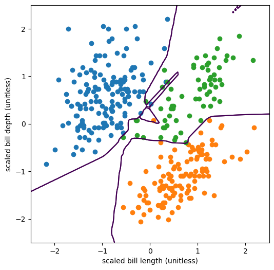
The optimizer used all of the parameters it had available to shrink-wrap the model around the training data. ReLU segments are carefully positioned to draw the decision boundary around every data point, sometimes even making islands to correctly categorize outlier penguins. This model is very overfitted.

The problem is that this model does not generalize. If we had more penguins to measure (sadly, we don’t), they probably wouldn’t line up with this decision boundary. There might be more orange (Gentoo) outliers in the region dominated by green (Chinstrap), but not likely in the same position as the outlier in this dataset, any islands this model might have drawn around the training-set outliers would be useless for categorizing new data.

What to do about it

First, you need a way to even know whether you’re under or overfitting. In the regression example, overlaying the fits on more data drawn from the same distribution revealed that the 0^th and 9^th degree polynomials are inaccurate/biased in some regions of \(x\). Judging a model by data that were not used to fit it is a powerful technique. In general, you’ll want to split your data into a subsample for training and another subsample reserved for validation and tests (which we’ll cover in a later section).

If you know that you’re underfitting a model, you can always add more parameters. That’s the benefit of neural networks over ansatz fits: if an ansatz is underfitting the data, then there are correlations in the data that you don’t know about. You need to fully understand them and put them in your fit function before you can make accurate predictions. But if a neural network is underfitting, just add more layers and/or more vector components per layer.

If you know that you’re overfitting a model, you could carefully scale back the number of parameters until it’s nearly minimal. We can think of an ML model like a scientific theory—this scaling back is like an application of Occam’s razor: you want the simplest model that fits the facts (data).

But what makes a model complex? You could count the number of parameters. It’s certainly the case that a Taylor polynomial with higher degree (more parameters) is more complex and more prone to overfitting than one with lower degree. There are also formal criteria, grounded in information theory like the Akaike Information Criterion (AIC), that count parameters. But in a neural network, is 1 hidden layer with 10 vector components more or less complex than 2 hidden layers with 5 components each? They do different things: remember that “one layer memorizes, many layers generalize.”

In the next section, we’ll see that there are “hands off” procedures for shrink-wrapping the complexity of a neural network until it has just enough freedom to describe a dataset and no more. These methods are called “regularization” and they’ve been used in linear fitting for decades.