Basic fitting#
In this section, we’ll start doing some computations, so get a Python interface (terminal, file, or notebook) handy! I’ll start with basic fitting, which I assume you’re familiar with, and show how neural networks are a generalization of linear fits.
Linear fitting#
Suppose you’re given a dataset in which pairs of values, \(x_i\) and \(y_i\) (indexes \(i \in [0, N)\) for \(N\) pairs), have an approximate linear relationship.
import numpy as np
import matplotlib.pyplot as plt
# uniformly random x values
x = np.random.uniform(-5, 5, 100)

# linear (2 * x + 3) plus normal-distributed noise
y = (2 * x + 3) + np.random.normal(0, 3, 100)
fig, ax = plt.subplots()

ax.scatter(x, y, marker="+", color="tab:orange")

plt.show()
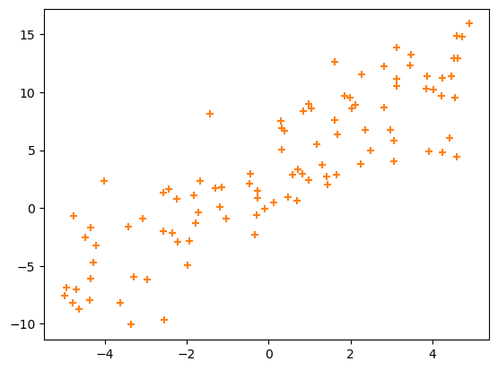
You can write an equation for an exact linear relationship:
and express the quality of this model as a fit to the data by how close it gets to the actual points:
If \(a\) and \(b\) are chosen well, the line will go through the middle of the points, like this:
\(\chi^2\) will be small because most \((a \, x_i + b)\) are close to the corresponding \(y_i\) and their squared difference will be small. You’re not given \(a\) and \(b\): you have to find \(a\) and \(b\) values that make \(\chi^2\) as small as possible. As it turns out, this problem can be solved with an exact formula:
sum1  = len(x)
sumx  = np.sum(x)
sumy  = np.sum(y)
sumxx = np.sum(x**2)
sumxy = np.sum(x * y)
delta = (sum1*sumxx) - (sumx*sumx)

a = ((sum1*sumxy) - (sumx*sumy))  / delta
b = ((sumxx*sumy) - (sumx*sumxy)) / delta
a, b
(np.float64(1.892749393195092), np.float64(2.9187036530258657))
which should be close to \(a = 2\) and \(b = 3\). Differences from the true values depend on the details of the noise. Regenerate the data points several times and you should see \(a\) jump around \(2\) and \(b\) jump around \(3\).
We can also confirm that the line goes through the points:
fig, ax = plt.subplots()

ax.scatter(x, y, marker="+", color="tab:orange")
ax.plot([-5, 5], [a*-5 + b, a*5 + b], color="tab:blue")

plt.show()
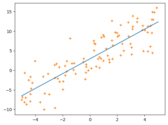
One thing that you should keep in mind is that we’re treating the \(x\) dimension and the \(y\) dimension differently: \(\chi^2\) is minimizing differences in predicted \(y\) (\(a x_i + b\)) and measured \(y\) (\(y_i\)): only the vertical differences between points and the line matter. In an experiment, you’d use \(x\) to denote the variables you can control, such as the voltage you apply to a circuit, and \(y\) is the measured response of the system, like a current in that circuit. In ML terminology, \(x\) is a “feature” and \(y\) is a “prediction,” and this whole fitting process is called “regression.”
Now suppose you control two features. The \(x\) values are now 2-dimensional vectors and you need a 2-dimensional \(a\) parameter to write a linear relationship:
where \(\cdot\) is matrix multiplication. This fits a plane in \(x^1\), \(x^2\) to 1-dimensional outputs \(y\).
Or suppose you have many feature dimensions:
and many predicted dimensions:
In this general case, you’re looking for a best-fit \(\hat{a}\) matrix and \(\vec{b}\) vector to describe a linear relationship between a set of n-dimensional vectors \(\vec{x}_i\) and a set of m-dimensional vectors \(\vec{y}_i\).
(By the way, it’s sometimes convenient to collect all of our free parameters, \(\hat{a}\) and \(\vec{b}\), into a single matrix \(\hat{A}\) by adding a “fake” dimension to the input features:
This is just a mathematical convenience that we’ll use below.)
Since this is still a linear fit and \(\chi^2\) is still ordinary least squares:
the solution is still an exact formula (see derivation):
where \(\hat{X}\) is a matrix of \(\vec{x}_i\) features with the “fake” dimension and \(\hat{Y}\) is a matrix of \(\vec{y}_i\) predictions. In general, you don’t need to use this equation directly, since there are libraries that compute linear fits. Scikit-Learn is one:
from sklearn.linear_model import LinearRegression
# Scikit-Learn wants an array of vectors, even if they're 1-dimensional
X = x.reshape(len(x), 1)   # or X = x[:, np.newaxis]
y = y

best_fit = LinearRegression().fit(X, y)

(a,) = best_fit.coef_
b = best_fit.intercept_

a, b
(np.float64(1.8927493931950918), np.float64(2.9187036530258657))
Or with more dimensions,
# uniformly random 2-D vectors
X = np.random.uniform(-5, 5, (100000, 2))

# true linear relationship (2-D → 3-D)
a_true = np.array([[1.1, 2.2],
                   [3.3, 4.4],
                   [5.5, 6.6]])
b_true = np.array([7.7, 8.8, 9.9])

# linear (a_true · x + b_true) for each x ∈ X plus noise
Y = (X @ a_true.T + b_true) + np.random.normal(0, 1, (100000, 3))
best_fit = LinearRegression().fit(X, Y)
best_fit.coef_
array([[1.09883189, 2.20101076],
       [3.29850983, 4.39957444],
       [5.50080438, 6.60116524]])
best_fit.intercept_
array([7.70133484, 8.80357903, 9.89906126])
Before we leave linear fitting, I want to point out that getting the indexes right is hard, and that both the mathematical notation and the array syntax hide this difficulty.
The first of the two fits with Scikit-Learn takes features (
X) with shape(100, 1)and targets (y) with shape(100,).The second takes features (
X) with shape(100000, 2)and targets (Y) with shape(100000, 3).
Scikit-Learn’s fit function is operating in two modes: the first takes a rank-1 array (the shape tuple has length 1) as a set of scalar targets and the second takes a rank-2 array as a set of vector targets. In both cases, Scikit-Learn requires the features to be rank-2, even if its second dimension just has length 1. (Why isn’t it just as strict about the targets? I don’t know.)
The mathematical notation is just as tricky: in the fully general case, we want to fit n-dimensional feature vectors \(\vec{x}_i\) to m-dimensional target vectors \(\vec{y}_i\), and we’re looking for a best-fit matrix \(\hat{A}\) (or a best-fit matrix \(\hat{a}\) and vector \(\vec{b}\), depending on whether we use the “fake dimension” trick or not). I’m using the word “vector” (with an arrow over the variable) to mean rank-1 and “matrix” (with a hat over the variable) to mean rank-2. Each pair of \(\vec{x}_i\) and \(\vec{y}_i\) vectors should be close to the
relationship and we minimize \(\chi^2\) for the whole dataset, summing over all \(i\).
This \(i\) can be thought of as another dimension, which is why we have a matrix \(\hat{X}\) and a matrix \(\hat{Y}\) (but still only a matrix \(\hat{A}\): the model parameters are not as numerous as the number of data points in the dataset).
In machine learning applications like computer vision, the individual data points are images, which we’d like to think of as having two dimensions. Thus, we can get into higher and higher ranks, and that’s why we usually talk about “tensors.” It will be worth paying special attention to which dimensions mean what. The notation gets complicated because it’s hard to decide where to put all those indexes. In the above, I’ve tried to consistently put the data-points-in-dataset index \(i\) as a subscript and the features/targets-are-vectors index as a superscript, but if we have more of them, then we just have to list them somehow.
A concept that you should not carry over from physics is the idea that tensors are defined by how they transform under spatial rotations—like the inertia tensor, the stress tensor, or tensors in general relativity. These “tensors” are just rectilinear arrays of numbers.
Non-linear fitting#
In physics, we usually try to find a first-principles theory that relates quantities \(x\) to measurements \(y\). Usually, that theory doesn’t predict a linear relationship. For example, the position of a tossed object as a function of time, \(y(t)\), is
where \(y_0\) and \(t_0\) are the starting position and time, and \(\mu\) and \(t_f\) are related to the air resistance.
def y_of_t(t):
    y0, t0, mu, tf = 60, 3, 0.05, 2
    return y0 - (1/mu)*np.log(np.cosh((t - t0)/tf))

def measurement_error(n):
    return np.random.normal(0, 1, n)
fig, ax = plt.subplots()

t = np.linspace(0, 10, 50)
y = y_of_t(t) + measurement_error(50)

ax.scatter(t, y, marker=".", color="tab:orange")
ax.errorbar(t, y, 1, fmt="none", color="tab:orange")

ax.set_xlabel("time after release")
ax.set_ylabel("height above ground")

plt.show()
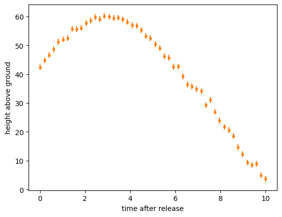
A linear fit would be a disaster:
best_fit = LinearRegression().fit(t[:, np.newaxis], y)

(linear_slope,) = best_fit.coef_
linear_intercept = best_fit.intercept_
fig, ax = plt.subplots()

ax.plot([0, 10], [linear_slope * 0 + linear_intercept, linear_slope * 10 + linear_intercept])

ax.scatter(t, y, marker=".", color="tab:orange")
ax.errorbar(t, y, 1, fmt="none", color="tab:orange")

ax.set_xlabel("time after release")
ax.set_ylabel("height above ground")

plt.show()
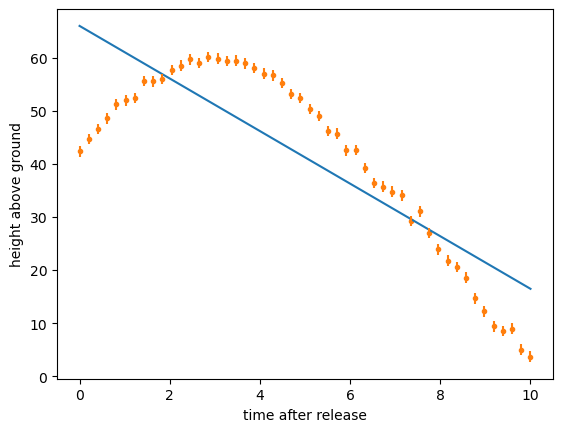
Instead, we use our theoretical knowledge of the shape of the functional form, often called an “ansatz,” and consider any unknown magnitudes as free parameters. Unlike a linear fit, there might not be an exact formula to find those parameters—there usually isn’t—so we use an algorithm to search the space of free parameters until it minimizes
In HEP, our favorite search algorithm is implemented by the Minuit library.
from iminuit import Minuit
from iminuit.cost import LeastSquares
def ansatz(t, y0, t0, mu, tf):
    return y0 - (1/mu)*np.log(np.cosh((t - t0)/tf))

least_squares = LeastSquares(t, y, 1, ansatz)
minimizer = Minuit(least_squares, y0=100, t0=0, mu=1, tf=5)   # <-- initial guess
minimizer.migrad()

y_from_ansatz = ansatz(t, **{p.name: p.value for p in minimizer.params})
fig, ax = plt.subplots()

ax.plot(t, y_from_ansatz)

ax.scatter(t, y, marker=".", color="tab:orange")
ax.errorbar(t, y, 1, fmt="none", color="tab:orange")

ax.set_xlabel("time after release")
ax.set_ylabel("height above ground")

plt.show()
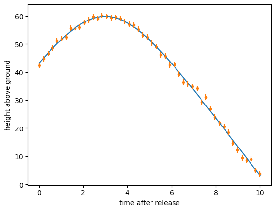
It’s a great fit, but you had to put part of the answer in to get this answer out. First, you had to know the functional form. Suppose you used the formula for the position of a tossed object without air resistance?
def wrong_ansatz(t, y0, t0, g):
    return y0 - (1/2)*g*(t - t0)**2

least_squares = LeastSquares(t, y, 1, wrong_ansatz)
minimizer = Minuit(least_squares, y0=100, t0=0, g=5)   # <-- initial guess
minimizer.migrad()

y_from_wrong_ansatz = wrong_ansatz(t, **{p.name: p.value for p in minimizer.params})
fig, ax = plt.subplots()

ax.plot(t, y_from_wrong_ansatz)

ax.scatter(t, y, marker=".", color="tab:orange")
ax.errorbar(t, y, 1, fmt="none", color="tab:orange")

ax.set_xlabel("time after release")
ax.set_ylabel("height above ground")

plt.show()
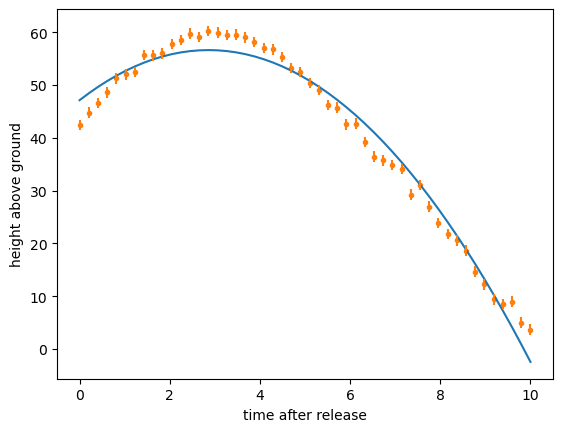
Or suppose you have the right functional form but provided the fitter with a bad initial guess? These are the numbers passed to the Minuit object constructor:
def ansatz(t, y0, t0, mu, tf):
    return y0 - (1/mu)*np.log(np.cosh((t - t0)/tf))

least_squares = LeastSquares(t, y, 1, ansatz)
minimizer = Minuit(least_squares, y0=100, t0=100, mu=100, tf=100)   # <-- initial guess
minimizer.migrad()

y_from_ansatz = ansatz(t, **{p.name: p.value for p in minimizer.params})
fig, ax = plt.subplots()

ax.plot(t, y_from_ansatz)

ax.scatter(t, y, marker=".", color="tab:orange")
ax.errorbar(t, y, 1, fmt="none", color="tab:orange")

ax.set_xlabel("time after release")
ax.set_ylabel("height above ground")

plt.show()
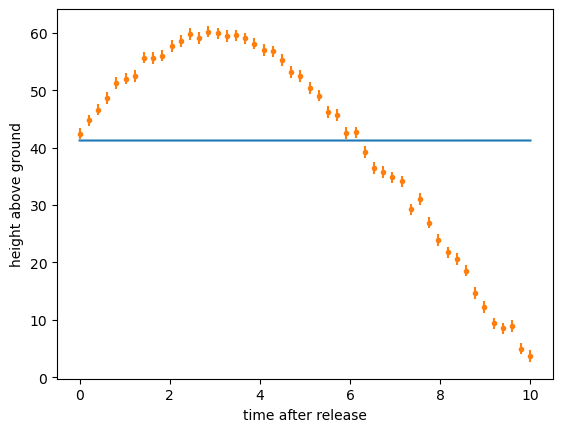
assert np.sum((y_from_ansatz - y)**2) > 100
The fit might converge to the wrong value or it might fail to converge entirely. (Long-time HEP experimentalists are familiar with these struggles!)
When to use basic fitting?#
If you do know enough to write a (correct) functional form and seed the fit with good starting values, then ansatz fitting is the best way to completely understand a system. Not only is the fitted function an accurate predictor of new values, but the parameters derived from the fit tell you about the underlying reality by filling in numerical values that were missing from the theory. In the above example, we could have used \(\mu\) and \(t_f\) to derive the force of air resistance on the tossed object—we’d learn something new. In general, all of physics is one big ansatz fit: we hypothesize general relativity and the Standard Model, then perform fits to measurements and learn the values of the constant of universal gravitation, the masses of quarks, leptons, and bosons, the strengths of interactions between them, etc. I didn’t show it in the examples above, but fitting procedures can also provide uncertainties on each parameter, their correlations, and likelihoods that the ansatz is correct.
However, most scientific problems beyond physics don’t have this much prior information. This is especially true in sciences that study the behavior of human beings. What is the underlying theory for a kid preferring chocolate ice cream over vanilla? What are the variables, and what’s the functional form? Even if you think that human behavior is determined by underlying chemistry and physics, it would be horrendously complex.
Here’s an example: the Boston Housing Prices is a classic dataset for regression. The goal is to predict median housing prices in towns around Boston using features like
per capita crime rate per town
proportion of residental land zoned for lots over 25,000 square feet
proportion of non-retail business acres per town
adjacency to the Charles River (a boolean variable)
nitric oxides concentration (parts per 10 million)
average number of rooms per dwelling
proportion of owner-occupied units built before 1940
weighted distances to 5 Boston employment centers
index of accessiblity to radial highways
full-value property-tax rate per $10,000
pupil-teacher ratio by town
\(1000(b - 0.63)^2\) where \(b\) is the proportion of Black residents
All of these seem like they would have an effect on housing prices, but it’s almost impossible to guess which would be more important. Problems like these are usually solved by a generic linear fit of many variables. Unimportant features would have a best-fit slope near zero, and if our goal is to find out which features are most important, we can force unimportant features toward zero with “regularization” (to be discussed in a later section). The idea of ML as “throw everything into a big fit” is close to what you have to do if you have no ansatz, and neural networks are a natural generalization of high-dimensional linear fitting.
In the next section, we’ll try to fit arbitrary non-linear curves without knowing an ansatz.
