Exercise 3: Classification

In this exercise, you’ll complete the previous section by performing a linear-logistic and full neural net classification of penguin species by bill length and depth, using PyTorch.

import numpy as np
import pandas as pd
import matplotlib.pyplot as plt

import torch
from torch import nn, optim

Get the data

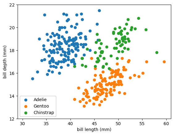
The code below is copied from the previous section. It loads the data and defines plotting functions to plot the data points and the 50% thresholds between categories.

penguins_df = pd.read_csv("data/penguins.csv")

categorical_int_df = penguins_df.dropna()[["bill_length_mm", "bill_depth_mm", "species"]]
categorical_int_df["species"], code_to_name = pd.factorize(categorical_int_df["species"].values)

categorical_1hot_df = pd.get_dummies(penguins_df.dropna()[["bill_length_mm", "bill_depth_mm", "species"]])

def plot_categorical_problem(ax, xlow=29, xhigh=61, ylow=12, yhigh=22):
    df_Adelie = categorical_1hot_df[categorical_1hot_df["species_Adelie"] == 1]
    df_Gentoo = categorical_1hot_df[categorical_1hot_df["species_Gentoo"] == 1]
    df_Chinstrap = categorical_1hot_df[categorical_1hot_df["species_Chinstrap"] == 1]

    ax.scatter(df_Adelie["bill_length_mm"], df_Adelie["bill_depth_mm"], color="tab:blue", label="Adelie")
    ax.scatter(df_Gentoo["bill_length_mm"], df_Gentoo["bill_depth_mm"], color="tab:orange", label="Gentoo")
    ax.scatter(df_Chinstrap["bill_length_mm"], df_Chinstrap["bill_depth_mm"], color="tab:green", label="Chinstrap")

    ax.set_xlim(xlow, xhigh)
    ax.set_ylim(ylow, yhigh)
    ax.set_xlabel("bill length (mm)")
    ax.set_ylabel("bill depth (mm)")

    ax.legend(loc="lower left", framealpha=1)

def plot_categorical_solution(ax, model, xlow=29, xhigh=61, ylow=12, yhigh=22):
    # compute the three probabilities for every 2D point in the background
    background_x, background_y = np.meshgrid(np.linspace(xlow, xhigh, 100), np.linspace(ylow, yhigh, 100))
    background_2d = np.column_stack([background_x.ravel(), background_y.ravel()])
    probabilities = model(background_2d)
    
    # draw contour lines where the probabilities cross the 50% threshold
    ax.contour(background_x, background_y, probabilities[:, 0].reshape(background_x.shape), [0.5])
    ax.contour(background_x, background_y, probabilities[:, 1].reshape(background_x.shape), [0.5])
    ax.contour(background_x, background_y, probabilities[:, 2].reshape(background_x.shape), [0.5])

fig, ax = plt.subplots()

plot_categorical_problem(ax)

plt.show()

Hints for the exercise

The linear-logistic fit has no hidden layer (no adaptive basis functions), just a linear fit that feeds into a softmax.

As a suggestion, build the model in two pieces:

model_without_softmax = nn.Sequential(
    nn.Linear(2, 3),         # 2D → 3D linear transformation
)

model_with_softmax = nn.Sequential(
    model_without_softmax,   # same 2D → 3D transformation
    nn.Softmax(dim=1),       # 3D space → 3 probabilities
)

Since nn.CrossEntropyLoss wants predictions without the softmax being applied and you’ll need to plot the result with the softmax applied.

These two models are connected:

list(model_without_softmax.parameters())

[Parameter containing:
 tensor([[-0.2326,  0.2633],
         [-0.0355,  0.4587],
         [-0.5658, -0.5759]], requires_grad=True),
 Parameter containing:
 tensor([-0.1672, -0.4778, -0.6891], requires_grad=True)]

list(model_with_softmax.parameters())

[Parameter containing:
 tensor([[-0.2326,  0.2633],
         [-0.0355,  0.4587],
         [-0.5658, -0.5759]], requires_grad=True),
 Parameter containing:
 tensor([-0.1672, -0.4778, -0.6891], requires_grad=True)]

They have the same parameter values, such that if model_without_softmax’s parameters are changed, you’ll see the same change in model_with_softmax.

I’ve found this linking of two model objects to be a useful way to keep track of whether the softmax has been applied—it’s in the name.

Also, you’ll need the data to be scaled before it reaches these parameters of order 1. You could either scale the data directly (and keep track of scaled and unscaled datasets) or make it a step in the model:

class ScaleFeatures(nn.Module):
    def __init__(self, means, stds):
        super().__init__()   # let PyTorch do its initialization first

        self.register_buffer("means", torch.tensor(means.reshape(1, 2), dtype=torch.float32))
        self.register_buffer("stds", torch.tensor(stds.reshape(1, 2), dtype=torch.float32))

    def __repr__(self):
        return f"{type(self).__name__}({self.means}, {self.stds})"

    def forward(self, x):
        return (x - self.means) / self.stds

scale_features = ScaleFeatures(
    categorical_int_df.drop(columns=["species"]).mean().values,
    categorical_int_df.drop(columns=["species"]).std().values,
)
scale_features

ScaleFeatures(tensor([[43.9928, 17.1649]]), tensor([[5.4687, 1.9692]]))

scaled_features = scale_features(
    torch.tensor(categorical_int_df.drop(columns=["species"]).values, dtype=torch.float32)
)
scaled_features[:15]

tensor([[-0.8947,  0.7796],
        [-0.8216,  0.1194],
        [-0.6753,  0.4241],
        [-1.3336,  1.0842],
        [-0.8581,  1.7444],
        [-0.9313,  0.3225],
        [-0.8764,  1.2366],
        [-0.5290,  0.2210],
        [-0.9861,  2.0491],
        [-1.7176,  1.9983],
        [-1.3518,  0.3225],
        [-0.9678,  0.9319],
        [-0.2730,  1.7952],
        [-1.7541,  0.6272],
        [ 0.3670,  2.2014]])

If your model works with scaled_features as input, it must not include scale_features as a step; if your model works with the original, unscaled features, then it must include scale_features as a step.

Finally, you’ll need to decide whether to use integer-encoded category labels (from categorical_int_df) as targets with dtype=torch.int64 or category probabilities (from categorical_1hot_df) as targets with dtype=torch.float32. nn.CrossEntropyLoss has wildly different behavior depending on the dtype of its input.

After the linear-logistic fit, add a 5-dimensional hidden layer with nn.ReLU activation functions. Remember that

relu = nn.ReLU()
relu

ReLU()

is an object that you can include in your model and

relu(scaled_features[:15])

tensor([[0.0000, 0.7796],
        [0.0000, 0.1194],
        [0.0000, 0.4241],
        [0.0000, 1.0842],
        [0.0000, 1.7444],
        [0.0000, 0.3225],
        [0.0000, 1.2366],
        [0.0000, 0.2210],
        [0.0000, 2.0491],
        [0.0000, 1.9983],
        [0.0000, 0.3225],
        [0.0000, 0.9319],
        [0.0000, 1.7952],
        [0.0000, 0.6272],
        [0.3670, 2.2014]])

is a function from tensors to tensors.

Have fun!