Neural networks#
In the previous section, we used adaptive basis functions to fit a generic shape and then noticed that this is a neural network with one hidden layer. This is not the usual way that neural networks are introduced.
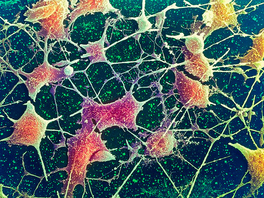
Originally, neural networks were inspired by analogy with neurons in the brain (hence the name). A neuron (nerve cell) receives \(n\) electro-chemical signals at one end and transmits \(m\) electro-chemical signals at the other end, according to some function.
Thus, we could write it like this:
which is
I personally don’t know whether real neurons are deterministic—can be modeled as a strict function of their inputs—or that it’s the same function \(f\) for all dendrites (\(y_i\)), but early formulations like McCulloch & Pitts (1943) used a sharp, binary step function:
hiding all the biological details in the sharpness of the step.
Perceptrons#
import numpy as np
import matplotlib.pyplot as plt
The first applications of neural networks as a computational tool were called “perceptrons.” Although Rosenblatt (1958) described a 3-layer neural network, a perceptron has come to be described as a 1-layer unit with a 1-dimensional output and a binary step function \(f\):
The 1-dimensional binary output is good for classification. A binary classification model is trained with a set of \(N\) data points, \(\vec{x}_i\) with \(i \in [0, N)\), and corresponding binary targets, \(y_i \in \{A, B\}\), to produce a predictor-machine that associates every point in the space \(\vec{x}\) with a probability that it is \(A\) or \(B\), \(P_A(\vec{x})\) and \(P_B(\vec{x})\). Naturally, \(P_A(\vec{x}) + P_B(\vec{x}) = 1\), so knowing \(P_A(\vec{x})\) is equivalent to knowing \(P_B(\vec{x})\).
Here’s a sample problem to learn: which regions of the plane are orange and which are blue?
blob1 = np.random.normal(0, 1, (1000, 2)) + np.array([[0, 3]])
blob2 = np.random.normal(0, 1, (1000, 2)) + np.array([[3, 0]])

shuffle = np.arange(len(blob1) + len(blob2))
np.random.shuffle(shuffle)

all_data = np.concatenate((blob1, blob2))[shuffle]
targets = np.concatenate((np.zeros(len(blob1)), np.ones(len(blob2))))[shuffle]
all_data
array([[ 2.68081828, -1.20869959],
       [ 0.85686947,  1.18276987],
       [ 0.87580754,  4.01273126],
       ...,
       [ 3.33845363,  0.4110794 ],
       [ 1.27433169,  2.4835029 ],
       [ 1.87698815, -1.74995476]])
targets
array([1., 0., 0., ..., 1., 0., 1.])
fig, ax = plt.subplots(figsize=(5, 5))

def plot_blob_points(ax, blob1, blob2):
    ax.scatter(blob1[:, 0], blob1[:, 1], marker=".", color="tab:blue")
    ax.scatter(blob2[:, 0], blob2[:, 1], marker=".", color="tab:orange")

plot_blob_points(ax, blob1, blob2)

ax.set_xlim(-4, 7)
ax.set_ylim(-4, 7)

plt.show()
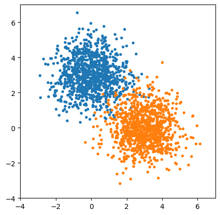
Since a perceptron doesn’t have a hidden layer, it’s not even considered a neural network by Scikit-Learn. A model consisting of a linear transformation passed into a sigmoid function is called logistic regression (sigmoid is sometimes called “logistic”).
from sklearn.linear_model import LogisticRegression
best_fit = LogisticRegression(penalty=None).fit(all_data, targets)
fig, ax = plt.subplots(figsize=(5, 5))

def plot_probability_and_50_threshold(ax, best_fit):
    # Compute the model's orange-vs-blue probability for 100×100 points in the background
    background_x, background_y = np.meshgrid(np.linspace(-4, 7, 100), np.linspace(-4, 7, 100))
    background_2d = np.column_stack((background_x.ravel(), background_y.ravel()))
    probabilities = best_fit.predict_proba(background_2d)

    # And draw a line where the probability crosses 0.5
    probability_of_0 = probabilities[:, 0].reshape(background_x.shape)
    ax.contour(background_x, background_y, probability_of_0, [0.5], linestyles=["--"])
    ax.contourf(background_x, background_y, probability_of_0, alpha=0.1)

plot_probability_and_50_threshold(ax, best_fit)
plot_blob_points(ax, blob1, blob2)

ax.set_xlim(-4, 7)
ax.set_ylim(-4, 7)

plt.show()
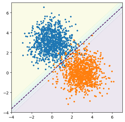
By drawing a line where \(P_A(\vec{x}) = 0.5\), we effectively turn the soft sigmoid boundary into a sharp binary classifier. LogisticRegression has a method to return this hard classification,
best_fit.predict([[0, 3]]).tolist()
[0.0]
best_fit.predict([[3, 0]]).tolist()
[1.0]
and a method to return the direct output of the logistic, which is the probability of each class:
best_fit.predict_proba([[0, 3]]).tolist()
[[0.9998169165408178, 0.00018308345918218523]]
best_fit.predict_proba([[3, 0]]).tolist()
[[0.00020939693195620723, 0.9997906030680438]]
best_fit.predict_proba([[2, 2]]).tolist()
[[0.5427903527016507, 0.4572096472983493]]
We’ve colored the plane by classification probability because the model makes a prediction for every infinitesimal point on the plane, though it was trained with finitely many points.
Some of the training points are on the wrong side of the 50% probability line, but the fitting process minimized these errors.
Now let’s consider a problem that perceptrons are bad at: distributions that are not linearly separable. Incidentally, this example started a controversy that was responsible for the first “winter” of AI (ref).
blobs1 = np.concatenate((
    np.random.normal(0, 1, (1000, 2)) + np.array([[0, 0]]),
    np.random.normal(0, 1, (1000, 2)) + np.array([[3, 3]]),
))
blobs2 = np.concatenate((
    np.random.normal(0, 1, (1000, 2)) + np.array([[0, 3]]),
    np.random.normal(0, 1, (1000, 2)) + np.array([[3, 0]]),
))

shuffle = np.arange(len(blobs1) + len(blobs2))
np.random.shuffle(shuffle)

all_data = np.concatenate((blobs1, blobs2))[shuffle]
targets = np.concatenate((np.zeros(len(blobs1)), np.ones(len(blobs2))))[shuffle]
best_fit = LogisticRegression(penalty=None).fit(all_data, targets)
fig, ax = plt.subplots(figsize=(5, 5))

plot_probability_and_50_threshold(ax, best_fit)
plot_blob_points(ax, blobs1, blobs2)

ax.set_xlim(-4, 7)
ax.set_ylim(-4, 7)

plt.show()
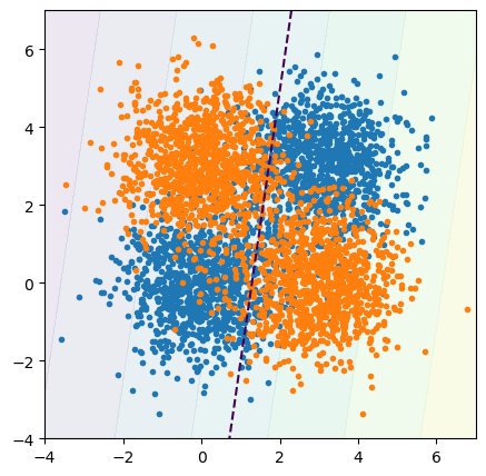
The 50% line is more-or-less random, and the probability threshold (gradient of background colors) isn’t as sharp. The trained model can’t make correct predictions for all 4 of the blob centers:
best_fit.predict([[0, 0], [3, 3]]).tolist() # should be the same as each other
[1.0, 0.0]
best_fit.predict([[0, 3], [3, 0]]).tolist() # should be the same as each other
[1.0, 0.0]
The reason should be clear by looking at the plot: there is no straight line that puts orange points on one side and blue points on the other. The model doesn’t have enough complexity to represent the data.
Adding a layer#
The solution starts with the observation that, in a brain, the output of one neuron feeds into the input of other neurons.
The full case of a general graph is hard to think about: what happens if the output of one neuron connects, perhaps through a series of other neurons, back to one of its own inputs? Since each \(x_i\) component is single-valued, a cycle has to be handled in a time-dependent way. A value of \(x_i = 0\) might, though some connections, force \(x_i \to 1\), but only at a later time.
There have been a few different approaches.
Require the graph to not have cycles. This is what McCulloch & Pitts did in their original formulation, since they were trying to build neuron diagrams that make logical propositions, like AND, OR, and NOT in digital circuits. These have clear inputs and outputs and should be time-independent.
Update the graph in discrete time-steps. If \(x_i = 0\) implies, through some connections, that \(x_i\) will be \(1\), it is updated in a later time-step.
The layers that we now use in most neural networks are a special case of #1. Even #2, which are known as Recurrent Neural Networks (RNNs), evolved toward a layered approach. Hopfield and Hinton’s 2024 Nobel prize work started with general, fully-connected graphs like the one below on the left, but eventually led to “Restricted Boltzmann machines,” in which nodes are separated into two types: visible (associated with observables to model) and hidden, with connections only between the visible and hidden, not within each type:
This is equivalent to the system of adaptive basis functions that we developed in the previous section:
Now let’s use it to classify orange and blue points, the problem described in the previous subsection.
from sklearn.neural_network import MLPRegressor
best_fit = MLPRegressor(
    activation="logistic", hidden_layer_sizes=(5,), max_iter=10000, alpha=0
).fit(all_data, targets)
fig, ax = plt.subplots(figsize=(5, 5))

def plot_probability_and_50_threshold_NN(ax, best_fit, low=-4, high=7):
    # MLPRegressor has a slightly different interface from LogisticRegressor,
    # so we need another plotting function. best_fit.predict returns probabilities.

    background_x, background_y = np.meshgrid(np.linspace(low, high, 100), np.linspace(low, high, 100))
    background_2d = np.column_stack((background_x.ravel(), background_y.ravel()))
    probabilities = best_fit.predict(background_2d)
    probability_of_0 = probabilities.reshape(background_x.shape)
    ax.contour(background_x, background_y, probability_of_0, [0.5], linestyles=["--"])
    ax.contourf(background_x, background_y, probability_of_0, alpha=0.1)

plot_probability_and_50_threshold_NN(ax, best_fit)
plot_blob_points(ax, blobs1, blobs2)

ax.set_xlim(-4, 7)
ax.set_ylim(-4, 7)

plt.show()
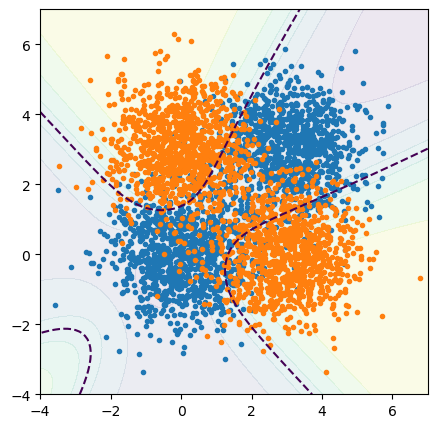
The shape of the boundary outside of the training data is unconstrained, but it’s allowed to curve enough to put orange points on one side and blue points on the other. It’s allowed to curve because we’ve given the fitter sigmoid-shaped adaptive basis functions to transform and add together (in 2 dimensions).
The basis functions didn’t have to be sigmoid-shaped. Here are a few common options:
Name |
Function |
|
|---|---|---|
binary step |
\(\displaystyle f(x) = \left\{\begin{array}{c l}0 & \mbox{if } x < 0 \\ 1 & \mbox{if } x \ge 0\end{array}\right.\) |
|
sigmoid, logistic, or soft step |
\(\displaystyle f(x) = \frac{1}{1 + e^{-x}}\) |
|
hyperbolic tangent |
\(\displaystyle f(x) = \frac{e^x - e^{-x}}{e^x + e^{-x}}\) |
|
rectified linear unit or ReLU |
\(\displaystyle f(x) = \left\{\begin{array}{c l}0 & \mbox{if } x < 0 \\ x & \mbox{if } x \ge 0\end{array}\right.\) |
|
leaky ReLU |
\(\displaystyle f(x) = \left\{\begin{array}{c l}\alpha x & \mbox{if } x < 0 \\ x & \mbox{if } x \ge 0\end{array}\right.\) |
|
sigmoid linear unit or swish |
\(\displaystyle f(x) = \frac{x}{1 + e^{-x}}\) |
Let’s use the ReLU shape instead. This is perhaps the most common activation function, because of its simplicity (and its derivatives don’t asymptotically approach zero).
best_fit = MLPRegressor(
    activation="relu", hidden_layer_sizes=(5,), max_iter=10000, alpha=0
).fit(all_data, targets)
fig, ax = plt.subplots(figsize=(5, 5))

plot_probability_and_50_threshold_NN(ax, best_fit)
plot_blob_points(ax, blobs1, blobs2)

ax.set_xlim(-4, 7)
ax.set_ylim(-4, 7)

plt.show()
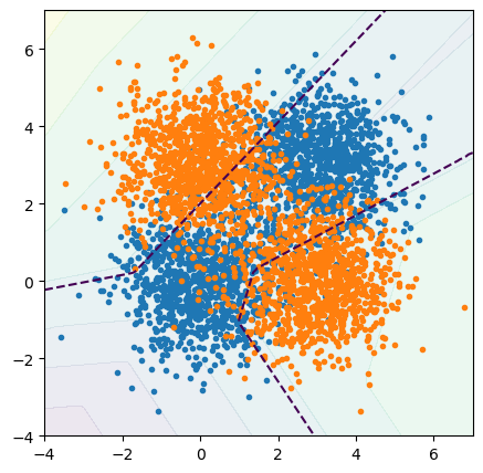
The boundaries still separate the orange and blue points, but now they’re made out of piecewise straight segments, not smooth curves.
Deep learning#
With enough components in the hidden layer, we can approximate any shape. After all, each component is one adaptive basis function, and our favorite activation functions (the table above) have one wiggle each. Adding a component to the hidden layer adds a wiggle, which the fitter can use to wrap around the training points.
However, if the fit function has too many wiggles to fit around the outliers in the training data, it will overfit the data (to be discussed in an upcoming section). We want a model that generalizes the training data, not one that memorizes it.
An effective way to do that is to add more hidden layers, like the diagram below:
\(\vec{x}^{L1}\) (layer 1) is the input and \(\vec{x}^{L2}\) (layer 2) is the first hidden layer. Then the output of that is passed through another linear transformation and activation function, as many times as we want. Each layer is a function composition. (Be careful when specifying how many layers a neural network has. We’re interested in how many linear transformations the network has, so we’d count the above as 4, not 5.)
This technique is called “deep learning” (especially when many, many layers are used) and it is largely responsible for the resurgence of interest in neural networks since 2015. Below is a plot of Google search volume for the words “neural network” and “deep learning”:
As you can see, interest in neural networks was waning in the early 2000’s, then there was a blip in theoretical interest in deep learning around 2009‒2010, followed by a rise in both after 2015. What happened was a combination of theoretical improvements and availability of GPUs. On the theory side:
2006: Hinton, Osindero, and Teh (ref) introduced a method to train one layer at a time to avoid the problem that deep layers “feel” less of a pull from training data (“vanishing gradients”).
2007: Bengio and LeCun (ref) demonstrated that networks with more than 2 or 3 layers can be applied to tasks that shallower networks can’t address without overfitting.
2007: Ranzato, Boureau, and LeCun (ref) presented a method to train deep networks in sparse batches.
Computationally, GPUs are very well suited to large-scale array operations. Both the hardware and the frameworks to use them became available at around this time. (CUDA was first released in 2006.)
But what really got things started was that deep neural networks started winning the ImageNet competition.
2012: AlexNet, a GPU-enabled 8 layer network (with ReLU), won ImageNet.
2015: ResNet, a GPU-enabled 152+ layer network (with skip-connections), won ImageNet.
Why deep learning?#
The general adage is that “one layer memorizes, many layers generalize.”
Each layer in a neural network is a function composition: the arbitrary curve that a set of adaptive basis functions learn is in a space that has already been transformed by a previous set of adaptive basis functions. Each layer warps space to make the next layer’s problem simpler.
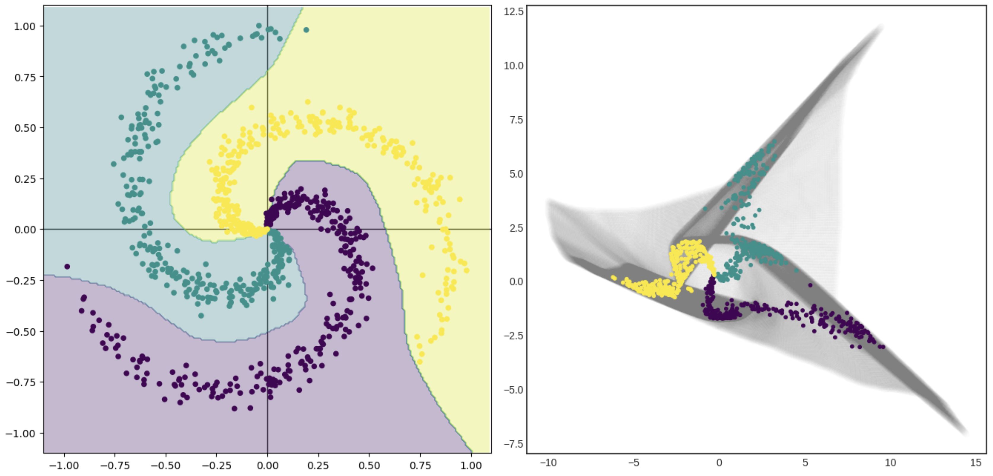
Roy Keyes has a fantastic demo (too much detail for this section) that classifies three categories of points that are arranged like spiral arms of a galaxy, shown below on the left. The first layer of the neural network transforms the \(x\)-\(y\) space of the original problem into the mesh shown in grey on the right. In the transformed space, the three spiral arms are now linearly separable. It is the starting point for the second layer.
For another illustration (ref), consider the horseshoe-shaped decision boundary below: it could be fit by a sufficiently large set of adaptive basis functions, with enough flexibility to account for each of the wiggles, but that would not take advantage of its symmetries. Two well-chosen folds make the symmetric parts overlap, and then it can be fitted by a simpler curve.
One hidden layer with many components has a lot of adjustable handles to fit a curve. Multiple hidden layers search for symmetries and try to use them to describe the data in a more generalizable way.
These arguments are heuristic: you could certainly have a problem with no internal symmetries. However, the fact that deep learning has been so successful might mean that most problems do.

