Exercise 2: Regression

Now that you’ve seen PyTorch used in a 1-dimensional regression problem, try converting from Scikit-Learn to PyTorch in this multidimensional problem.

import numpy as np
import pandas as pd
import matplotlib.pyplot as plt

Boston House Prices dataset

I previously mentioned the Boston House Prices dataset. It contains descriptive details about towns around Boston:

• CRIM: per capita crime rate per town

• ZN: proportion of residental land zoned for lots over 25,000 square feet

• INDUS: proportion of non-retail business acres per town

• CHAS: adjacency to the Charles River (a boolean variable)

• NOX: nitric oxides concentration (parts per 10 million)

• RM: average number of rooms per dwelling

• AGE: proportion of owner-occupied units built before 1940

• DIS: weighted distances to 5 Boston employment centers

• RAD: index of accessiblity to radial highways

• TAX: full-value property-tax rate per $10,000

• PTRATIO: pupil-teacher ratio by town

• B: \(1000(b - 0.63)^2\) where \(b\) is the proportion of Black residents

• LSTAT: % lower status by population

as well as MEDV, the median prices of owner-occupied homes. Your job is to predict the prices, given all of the other data as features. You will do this with both a linear fit and a neural network with 5 hidden sigmoid components.

You can get the dataset from the original source or from this project’s GitHub: deep-learning-intro-for-hep/data/boston-house-prices.csv.

housing_df = pd.read_csv(
    "data/boston-house-prices.csv", sep="\s+", header=None,
    names=["CRIM", "ZN", "INDUS", "CHAS", "NOX", "RM", "AGE", "DIS", "RAD", "TAX", "PTRATIO", "B", "LSTAT", "MEDV"],
)
housing_df

	CRIM	ZN	INDUS	CHAS	NOX	RM	AGE	DIS	RAD	TAX	PTRATIO	B	LSTAT	MEDV
0	0.00632	18.0	2.31	0	0.538	6.575	65.2	4.0900	1	296.0	15.3	396.90	4.98	24.0
1	0.02731	0.0	7.07	0	0.469	6.421	78.9	4.9671	2	242.0	17.8	396.90	9.14	21.6
2	0.02729	0.0	7.07	0	0.469	7.185	61.1	4.9671	2	242.0	17.8	392.83	4.03	34.7
3	0.03237	0.0	2.18	0	0.458	6.998	45.8	6.0622	3	222.0	18.7	394.63	2.94	33.4
4	0.06905	0.0	2.18	0	0.458	7.147	54.2	6.0622	3	222.0	18.7	396.90	5.33	36.2
...	...	...	...	...	...	...	...	...	...	...	...	...	...	...
501	0.06263	0.0	11.93	0	0.573	6.593	69.1	2.4786	1	273.0	21.0	391.99	9.67	22.4
502	0.04527	0.0	11.93	0	0.573	6.120	76.7	2.2875	1	273.0	21.0	396.90	9.08	20.6
503	0.06076	0.0	11.93	0	0.573	6.976	91.0	2.1675	1	273.0	21.0	396.90	5.64	23.9
504	0.10959	0.0	11.93	0	0.573	6.794	89.3	2.3889	1	273.0	21.0	393.45	6.48	22.0
505	0.04741	0.0	11.93	0	0.573	6.030	80.8	2.5050	1	273.0	21.0	396.90	7.88	11.9

506 rows × 14 columns

The MEDV column is the prediction target; all the rest of the columns are features.

Linear solution in Scikit-Learn

As before, we get the LinearRegression fitter from Scikit-Learn:

from sklearn.linear_model import LinearRegression

regression_features = housing_df.drop(columns=["MEDV"]).values
regression_targets = housing_df["MEDV"].values

regression_features.shape, regression_targets.shape

((506, 13), (506,))

best_fit = LinearRegression().fit(regression_features, regression_targets)

best_fit.coef_

array([-1.08011358e-01,  4.64204584e-02,  2.05586264e-02,  2.68673382e+00,
       -1.77666112e+01,  3.80986521e+00,  6.92224640e-04, -1.47556685e+00,
        3.06049479e-01, -1.23345939e-02, -9.52747232e-01,  9.31168327e-03,
       -5.24758378e-01])

best_fit.intercept_

np.float64(36.459488385089955)

The algorithm says that’s the best fit, but don’t be satisfied without looking at it somehow. The 13-dimensional feature space is too large to plot directly, but we have to plot something!

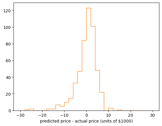
How about the residuals, the difference between the predicted prices and the actual prices?

fig, ax = plt.subplots()

linear_fit_residuals = best_fit.predict(regression_features) - regression_targets

ax.hist(linear_fit_residuals, bins=30, range=(-30, 30), histtype="step", color="tab:orange")

ax.set_xlabel("predicted price - actual price (units of $1000)")

plt.show()

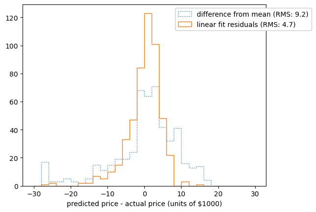
Fine, but you still don’t know if you’ve done anything. What should the residuals plot look like? Has the fit improved anything?

If the linear fit gives us a narrower residuals distribution than a simpler model, such as “given only the average housing price, assume that the price is equal to the average” (a 1-parameter model), then at least we know that the linear model is a step in the right direction.

fig, ax = plt.subplots()

difference_from_mean = regression_targets.mean()- regression_targets
linear_fit_residuals = best_fit.predict(regression_features) - regression_targets

ax.hist(difference_from_mean, bins=30, range=(-30, 30), histtype="step", ls=":",
        label=f"difference from mean (RMS: {np.sqrt(difference_from_mean.var()):.2g})")
ax.hist(linear_fit_residuals, bins=30, range=(-30, 30), histtype="step",
        label=f"linear fit residuals (RMS: {np.sqrt(linear_fit_residuals.var()):.2g})")

ax.set_xlabel("predicted price - actual price (units of $1000)")
ax.legend(loc="upper right", bbox_to_anchor=(1.2, 1), framealpha=1)

plt.show()

Neural network solution in Scikit-Learn

Okay, now what about a neural network? We can use Scikit-Learn’s MLPRegressor.

from sklearn.neural_network import MLPRegressor

But remember that neural networks are initialized with weights of order 1, so the regression features (which have different scales for each column) and targets should be adjusted to be of order 1 before passing them into the fitter.

Note that np.mean and np.std with axis=0 take the mean and standard deviation over the 506 rows, rather than the 13 columns.

When we make predictions with the model, they’ll be in this scaled space, so we’ll need to unscale them to meaningfully compare them with the original targets. (This is part of the “leaky abstraction” of machine learning models: you just have to know which level of transformation a model has been trained for and use it accordingly. Python doesn’t see the difference between unscaled numbers and scaled numbers and can’t give you a TypeError when you use the wrong one.)

regression_features_scaled = (
    regression_features - regression_features.mean(axis=0)
) / regression_features.std(axis=0)

regression_targets_scaled = (
    regression_targets - regression_targets.mean()
) / regression_targets.std()

def unscale_predictions(predictions):
    return (predictions * regression_targets.std()) + regression_targets.mean()

In this neural network, let’s use 5 sigmoids (“logistic” functions) in the hidden layer. The alpha=0 turns off regularization, which we haven’t covered yet.

best_fit_nn = MLPRegressor(
    activation="logistic", hidden_layer_sizes=(5,), solver="lbfgs", max_iter=10000, alpha=0
).fit(regression_features_scaled, regression_targets_scaled)

fig, ax = plt.subplots()

neural_network_residuals = unscale_predictions(best_fit_nn.predict(regression_features_scaled)) - regression_targets

ax.hist(difference_from_mean, bins=30, range=(-30, 30), histtype="step", ls=":",
        label=f"difference from mean (RMS: {np.sqrt(difference_from_mean.var()):.2g})")
ax.hist(linear_fit_residuals, bins=30, range=(-30, 30), histtype="step",
        label=f"linear fit residuals (RMS: {np.sqrt(linear_fit_residuals.var()):.2g})")
ax.hist(neural_network_residuals, bins=30, range=(-30, 30), histtype="step",
        label=f"neural network residuals: (RMS: {np.sqrt(neural_network_residuals.var()):.2g})")

ax.set_xlabel("predicted price - actual price (units of $1000)")
ax.legend(loc="upper right", bbox_to_anchor=(1.2, 1), framealpha=1)

plt.show()

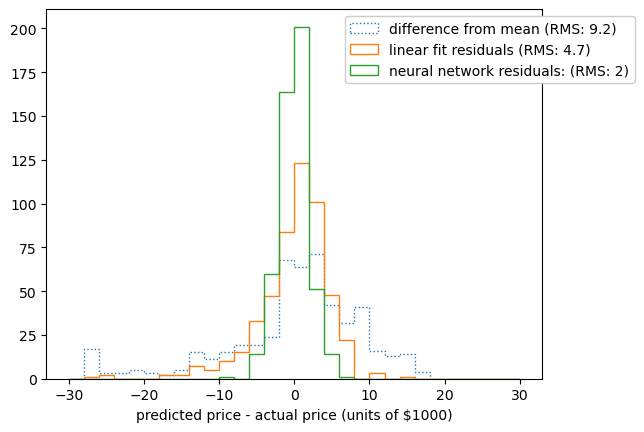
The neural network is a further improvement, beyond the linear model. This shouldn’t be a surprise, since we’ve given the fitter more knobs to turn: instead of just a linear transformation, we have a linear transformation followed by 5 adaptive basis functions (the sigmoids).

Note that this is not a proper procedure for modeling yet: you can get an arbitrarily good fit by adding more and more sigmoids. Try replacing the (5,) with (100,) to see what happens to the neural network residuals. If we have enough adaptive basis functions, we can center one on every input data point, and our “quality check” is looking at the model’s prediction of those same input data points. We’ll talk more about this in the sections on overfitting and splitting data into training, validation, and test datasets.

Now do it in PyTorch

Your job is to reproduce the linear fit and the neural network in PyTorch. Some things to watch out for:

• You have to scale the inputs and outputs. Whereas Scikit-Learn uses an exact formula in its LinearRegression, PyTorch doesn’t handle linear fits as a special case. Its optimizers will take small, iterative steps from the initial weights of order 1, so you’d either need to run for many epochs or help it out by posing a problem with order 1 values.

• If you use PyTorch’s optim.LBFGS, note that you can’t write a simple for loop, as you would with any other optimizer. This optimizer has to partly control its iteration, so you have to call it through its step method:

optimizer = optim.LBFGS(model.parameters())

def what_would_go_into_the_for_loop():
    # tell the optimizer to begin an optimization step
    optimizer.zero_grad()

    # use the model as a prediction function: features → prediction
    predictions = model(tensor_features)

    # compute the loss (χ²) between these predictions and the intended targets
    loss = loss_function(predictions, tensor_targets)

    # tell the loss function to end an optimization step
    loss.backward()

for epoch in range(number_of_epochs):
    optimizer.step(what_would_go_into_the_for_loop)

• You don’t have to use the same optimizer as Scikit-Learn (though you might need more epochs to reach the same solution). However, be sure to use the same sigmoid (“logistic”) activation function and number of hidden layer components, so that the results are comparable.

• To debug, print out individual values! Make plots! Look at all the pieces, even when things seem to be going well.

Good luck!