Feature selection and “the kernel trick”

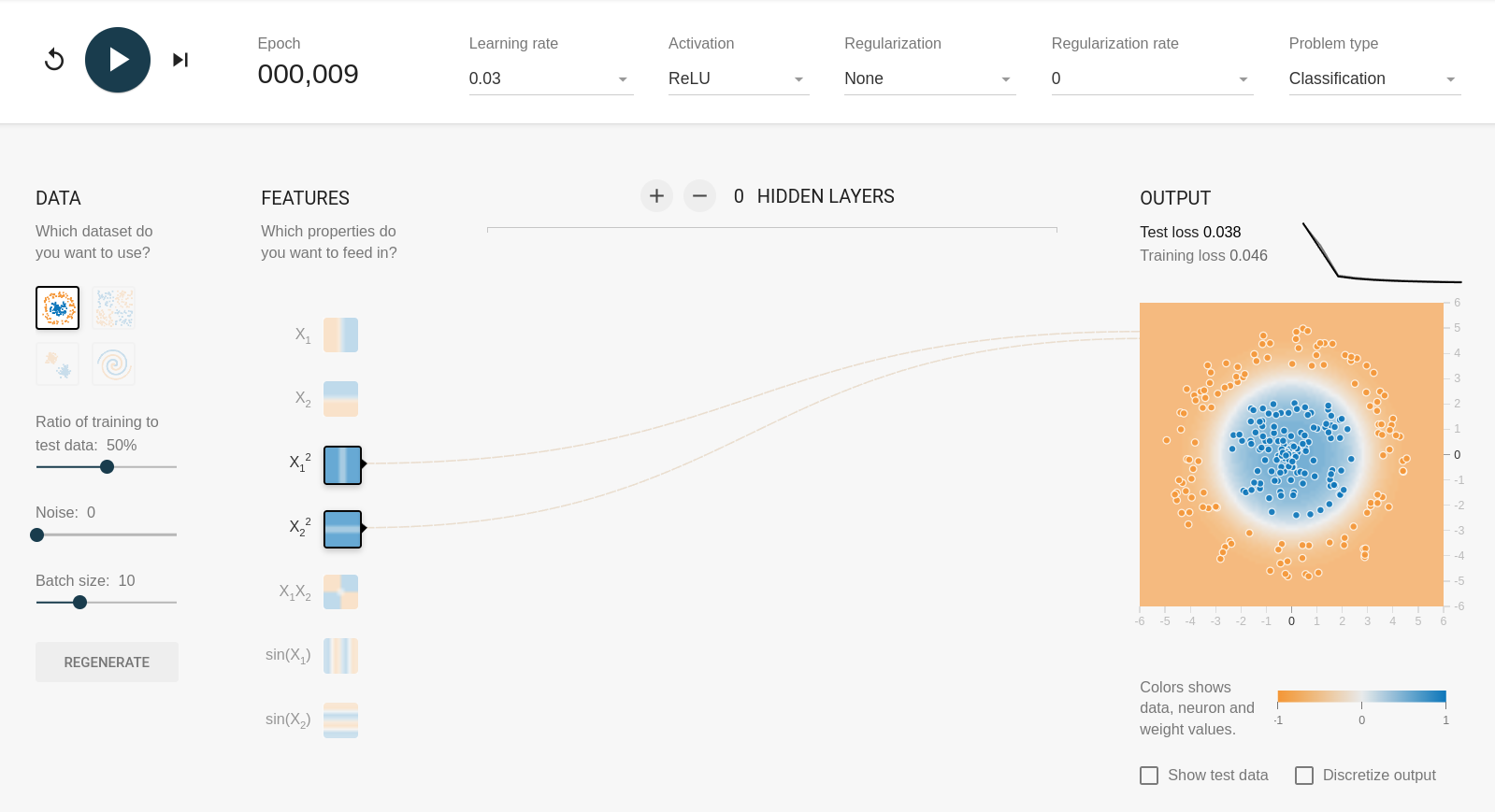
In playground.tensorflow.org, you could build the model with mathematical combinations of the input features, \(x_1\) and \(x_2\), rather than just the features themselves. For example, the circle problem can be solved without any hidden layers if the features are \({x_1}^2\) and \({x_2}^2\):

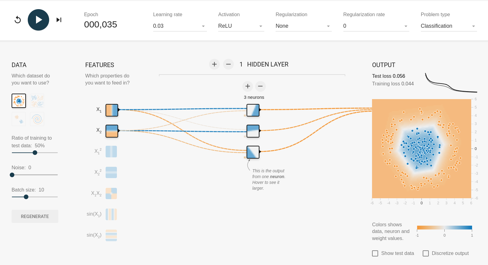
But with \(x_1\) and \(x_2\) as input features, it needs at least 3 components in a hidden layer:

Without hidden layers, the fit is purely linear: the first fit works because a circle centered on \(x_1 = x_2 = 0\) is a threshold in \({x_1}^2 + {x_2}^2\). Similarly, the xor problem can be solved with \(x_1 x_2\) and nothing else: the fit is a single linear term!

The general technique of making a linear classifier solve non-linear problems by giving it non-linear combinations of features was called “the kernel trick,” and it’s most strongly associated with Support Vector Machines (SVMs). SVMs were popular as an alternative to neural networks in the late 1990’s and early 2000’s; the kernel trick made up for the fact that an SVM is a linear classifier. However, we can just as easily use it to extend the expressiveness of a non-linear classifier.

import numpy as np
import matplotlib.pyplot as plt

Space of feature combinations

Let’s demonstrate this by recreating the circle problem and its solution, using Scikit-Learn’s LogisticRegression (which is a linear fit followed by a sigmoid).

inner_r = abs(np.random.normal(0, 1, 1000))
outer_r = abs(np.random.normal(3, 0.5, 1000))
inner_phi = np.random.uniform(0, 2*np.pi, 1000)
outer_phi = np.random.uniform(0, 2*np.pi, 1000)

inner_x1 = inner_r * np.cos(inner_phi)
inner_x2 = inner_r * np.sin(inner_phi)
outer_x1 = outer_r * np.cos(outer_phi)
outer_x2 = outer_r * np.sin(outer_phi)

shuffle = np.arange(len(inner_x1) + len(outer_x1))
np.random.shuffle(shuffle)

all_x1 = np.concatenate([inner_x1, outer_x1])[shuffle]
all_x2 = np.concatenate([inner_x2, outer_x2])[shuffle]
targets = np.concatenate([np.zeros(1000), np.ones(1000)])[shuffle]

features_linear = np.column_stack([all_x1, all_x2])
features_linear

array([[-2.1871252 , -2.92091133],
       [ 0.06169389, -0.19121885],
       [-0.76407685,  2.98128673],
       ...,
       [-0.16998335,  0.14582067],
       [ 2.49576316,  2.8501664 ],
       [-1.67434432,  0.06226052]])

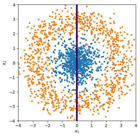
A linear fit in \(x\), \(y\) can’t find the decision boundary because it’s intrinsically non-linear.

from sklearn.linear_model import LogisticRegression

best_fit = LogisticRegression(penalty=None).fit(features_linear, targets)

fig, ax = plt.subplots(figsize=(5, 5))

def plot_threshold(ax, model_of_x1x2):
    background_x1, background_x2 = np.meshgrid(np.linspace(-4, 4, 100), np.linspace(-4, 4, 100))
    background_x1x2 = np.column_stack([background_x1.ravel(), background_x2.ravel()])
    ax.contour(background_x1, background_x2, model_of_x1x2(background_x1x2)[:, 0].reshape(background_x1.shape), [0.5], linewidths=[4])

def plot_points(ax):
    ax.scatter(inner_x1, inner_x2, marker=".")
    ax.scatter(outer_x1, outer_x2, marker=".")
    ax.set_xlim(-4, 4)
    ax.set_ylim(-4, 4)
    ax.set_xlabel("$x_1$")
    ax.set_ylabel("$x_2$")

plot_threshold(ax, lambda x1x2: best_fit.predict_proba(x1x2))
plot_points(ax)

plt.show()

But if our features are \({x_1}^2\) and \({x_2}^2\),

features_quadratic = np.column_stack([all_x1**2, all_x2**2])
features_quadratic

array([[4.78351666e+00, 8.53172301e+00],
       [3.80613631e-03, 3.65646493e-02],
       [5.83813425e-01, 8.88807056e+00],
       ...,
       [2.88943384e-02, 2.12636664e-02],
       [6.22883377e+00, 8.12344849e+00],
       [2.80342890e+00, 3.87637206e-03]])

best_fit = LogisticRegression(penalty=None).fit(features_quadratic, targets)

fig, ax = plt.subplots(figsize=(5, 5))

plot_threshold(ax, lambda x1x2: best_fit.predict_proba(x1x2**2))
plot_points(ax)

plt.show()

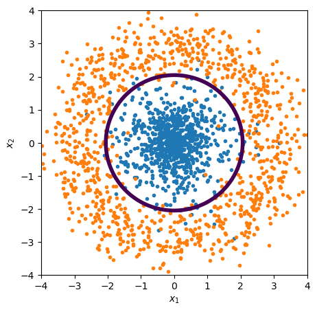
The fact that this discriminator is linear is more obvious if we actually plot the space of \({x_1}^2\) and \({x_2}^2\):

fig, ax = plt.subplots(figsize=(5, 5))

model_of_x1x2squared = lambda x1x2squared: best_fit.predict_proba(x1x2squared)

background_x1squared, background_x2squared = np.meshgrid(np.linspace(0, 16, 100), np.linspace(0, 16, 100))
background_x1x2squared = np.column_stack([background_x1squared.ravel(), background_x2squared.ravel()])
ax.contour(
    background_x1squared,
    background_x2squared,
    model_of_x1x2squared(background_x1x2squared)[:, 0].reshape(background_x1squared.shape),
    [0.5],
    linewidths=[4],
)

ax.scatter(inner_x1**2, inner_x2**2, marker=".")
ax.scatter(outer_x1**2, outer_x2**2, marker=".")
ax.set_xlim(0, 16)
ax.set_ylim(0, 16)
ax.set_xlabel("${x_1}^2$")
ax.set_ylabel("${x_2}^2$")

plt.show()

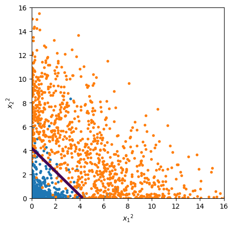
Usually, we don’t know exactly which features are best for a given problem, such as \({x_1}^2\) and \({x_2}^2\) for a circle centered on zero. In the general case, we’d add polynomial combinations of the basic features, such as \({x_1}^2\), \({x_2}^2\), \({x_1} {x_2}\) for 2^nd degree, \({x_1}^3\), \({x_2}^3\), \({x_1}^2 {x_2}\), \({x_1} {x_2}^2\) for 3^rd degree, etc.

Let’s do one last example with the circle problem: fit it in the 3-dimensional space of \(x_1\), \(x_2\), \({x_1}^2 + {x_2}^2\):

features_3d = np.column_stack([all_x1, all_x2, all_x1**2 + all_x2**2])
features_3d

array([[-2.1871252 , -2.92091133, 13.31523967],
       [ 0.06169389, -0.19121885,  0.04037079],
       [-0.76407685,  2.98128673,  9.47188399],
       ...,
       [-0.16998335,  0.14582067,  0.050158  ],
       [ 2.49576316,  2.8501664 , 14.35228226],
       [-1.67434432,  0.06226052,  2.80730527]])

best_fit = LogisticRegression(penalty=None).fit(features_3d, targets)

fig, ax = plt.subplots(figsize=(5, 5))

def model_of_x1x2(x1x2):
    x1 = x1x2[:, 0]
    x2 = x1x2[:, 1]
    everything = np.column_stack([x1, x2, x1**2 + x2**2])
    return best_fit.predict_proba(everything)

plot_threshold(ax, model_of_x1x2)
plot_points(ax)

plt.show()

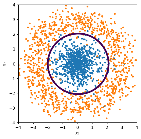
Now tilt the space so that we can see how the points extend in the 3^rd dimension, \({x_1}^2 + {x_2}^2\):

fig = plt.figure(figsize=(6, 6))
ax = fig.add_subplot(111, projection="3d")
ax.set_box_aspect(None, zoom=1.25)
ax.view_init(elev=3, azim=30)

ax.scatter(features_3d[targets == 0, 0], features_3d[targets == 0, 1], zs=features_3d[targets == 0, 2], marker=".")
ax.scatter(features_3d[targets == 1, 0], features_3d[targets == 1, 1], zs=features_3d[targets == 1, 2], marker=".")

background_x1, background_x2 = np.meshgrid(np.linspace(-4, 4, 2), np.linspace(-4, 4, 2))
ax.plot_surface(background_x1, background_x2, np.full_like(background_x1, 3.63636364), facecolors=["green"], alpha=0.1)

ax.set_xlabel("$x_1$")
ax.set_ylabel("$x_2$")
ax.set_zlabel("${x_1}^2 + {x_2}^2$")

plt.show()

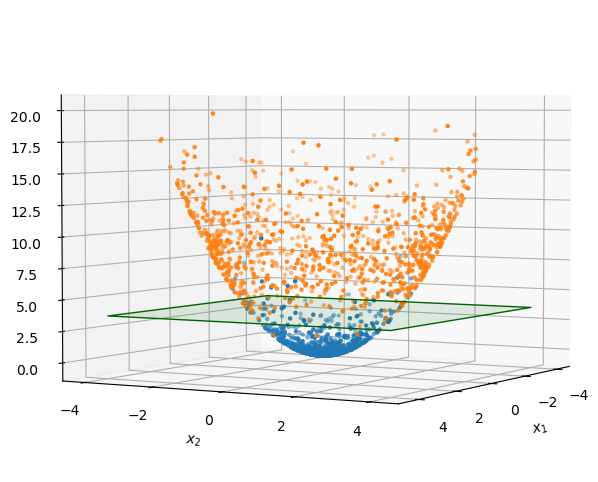
Since the 3^rd dimension is a strict function of the first 2, the data points are all on a surface, and the surface curves in such a way as to make the plane effective at separating orange points from blue points.

Taylor and Fourier series as kernel trick

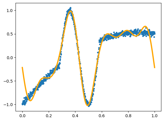
Before introducing adaptive basis functions, I argued that Taylor and Fourier series are essentially linear fits. This is because they’re also applications of the kernel trick, taken to a high degree.

Let’s demonstrate it with the crazy function from the section on Universal Approximators:

\[\begin{split}y = \left\{\begin{array}{l l} \sin(22 x) & \mbox{if } |x - 0.43| < 0.15 \\ -1 + 3.5 x - 2 x^2 & \mbox{otherwise} \\ \end{array}\right.\end{split}\]

def truth(x):
    return np.where(abs(x - 0.43) < 0.15, np.sin(22*x), -1 + 3.5*x - 2*x**2)

x = np.linspace(0, 1, 1000)[:, np.newaxis]
y = truth(x)[:, 0] + np.random.normal(0, 0.03, 1000)

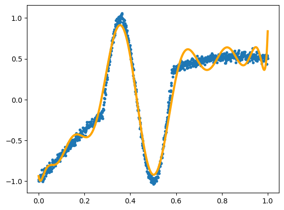
For each value in the array x, we compute \(x^0\), \(x^1\), \(x^2\), …, \(x^{14}\). Instead of 1 feature, \(x\), this fit has 15 input features.

polynomial_features = np.hstack([x**i for i in range(15)])
polynomial_features.shape

(1000, 15)

But it’s still linear. (fit_intercept=False because we already have a term for \(x^0 = 1\).)

from sklearn.linear_model import LinearRegression

best_fit = LinearRegression(fit_intercept=False).fit(polynomial_features, y)

fig, ax = plt.subplots()

ax.scatter(x, y, marker=".")
ax.plot(x, best_fit.predict(polynomial_features), color="orange", linewidth=3)

plt.show()

Now for Fourier terms:

cos_components = [np.cos(2*np.pi * i * x) for i in range(1, 8)]
sin_components = [np.sin(2*np.pi * i * x) for i in range(1, 8)]

fourier_features = np.hstack([np.ones_like(x)] + cos_components + sin_components)
fourier_features.shape

(1000, 15)

best_fit = LinearRegression(fit_intercept=False).fit(fourier_features, y)

fig, ax = plt.subplots()

ax.scatter(x, y, marker=".")
ax.plot(x, best_fit.predict(fourier_features), color="orange", linewidth=3)

plt.show()

But we can’t do that with the adaptive basis functions.

Feature engineering

This process of choosing relevant combinations of input variables and adding them to a model as features is sometimes called “feature engineering.” If you know what features are relevant, as in the circle problem, then computing them explicitly as inputs will improve the fit and its generalization. If you’re not sure, including them in the mix with the basic features can only help the model find a better optimum (possibly by overfitting; see the next section). The laundry list of features in the Boston House Prices dataset is an example of feature engineering.

Sometimes, feature engineering is presented as a bad thing, since you, as data analyst, are required to be more knowledgeable about the details of the problem. The ML algorithm isn’t “figuring it out for you.” That’s a reasonable perspective if you’re developing ML algorithms and you want them to apply to any problem, regardless of how deeply understood those problems are. It’s certainly impressive when an ML algorithm rediscovers features we knew were important or discovers new ones. However, if you’re a data analyst, trying to solve one particular problem, and you happen to know about some relevant features, it’s in your interest to include them in the mix!

Sometimes, incorporating domain-specific knowledge in the ML model is presented as a good thing—not just feature engineering, but at all levels. For example, Physics-Informed Neural Networks (PINN) incorporate conservation laws and boundary conditions into the loss function instead of rediscovering such constraints from the data. ML developments seem to hop-scotch between increasing generality and increasing specificity.

In setting up your ML procedure, be clear about your own goals: how much information do you already have and how much do you want the model to discover on its own? What expressions or constraints are easy for you to write down, which do you need help with, and what might be completely unknown, latent in the data?

If you add too many features and the model overfits, there are ways of dealing with that.