Classification in PyTorch

This is a continuation of the previous section, introducing PyTorch for two basic problems: regression and classification.

import numpy as np
import pandas as pd
import matplotlib.pyplot as plt

Penguins again!

See Regression in PyTorch for instructions on how to get the data.

penguins_df = pd.read_csv("data/penguins.csv")
penguins_df

	species	island	bill_length_mm	bill_depth_mm	flipper_length_mm	body_mass_g	sex	year
0	Adelie	Torgersen	39.1	18.7	181.0	3750.0	male	2007
1	Adelie	Torgersen	39.5	17.4	186.0	3800.0	female	2007
2	Adelie	Torgersen	40.3	18.0	195.0	3250.0	female	2007
3	Adelie	Torgersen	NaN	NaN	NaN	NaN	NaN	2007
4	Adelie	Torgersen	36.7	19.3	193.0	3450.0	female	2007
...	...	...	...	...	...	...	...	...
339	Chinstrap	Dream	55.8	19.8	207.0	4000.0	male	2009
340	Chinstrap	Dream	43.5	18.1	202.0	3400.0	female	2009
341	Chinstrap	Dream	49.6	18.2	193.0	3775.0	male	2009
342	Chinstrap	Dream	50.8	19.0	210.0	4100.0	male	2009
343	Chinstrap	Dream	50.2	18.7	198.0	3775.0	female	2009

344 rows × 8 columns

This time, we’re going to focus on the categorical variables, species, island, sex, and year.

Numerical and categorical data

Numerical versus categorical may be thought of as data types in a programming language: integers and floating-point types are numerical, booleans and strings are categorical. However, they can also be thought of as the fundamental types in data analysis, which determines which set of mathematical operations are meaningful:

Level	Math	Description	Physics example
Nominal category	=, ≠	categories without order	jet classification, data versus Monte Carlo
Ordinal category	>, <	categories that have an order	barrel region, overlap region, endcap region
Interval number	+, ‒	doesn’t have an origin	energy, voltage, position, momentum
Ratio number	×, /	has an origin	absolute temperature, mass, opening angle

Python’s TypeError won’t tell you if you’re inappropriately multiplying or dividing an interval number, but it will tell you if you try to subtract strings.

Categorical problems involve at least one categorical variable. For instance, given a penguin’s bill length and bill depth, what’s its species? We might ask a categorical model to predict the most likely category or we might ask it to tell us the probabilities of each category.

We can’t pass string-valued variables into a fitter, so we need to convert the strings into numbers. Since these categories are nominal (not ordinal), equality/inequality is the only meaningful operation, so the numbers should only indicate which strings are the same as each other and which are different.

Pandas has a function, pd.factorize, to turn unique categories into unique integers and an index to get the original strings back. (You can also use Pandas’s categorical dtype.)

categorical_int_df = penguins_df.dropna()[["bill_length_mm", "bill_depth_mm", "species"]]
categorical_int_df["species"], code_to_name = pd.factorize(categorical_int_df["species"].values)
categorical_int_df

	bill_length_mm	bill_depth_mm	species
0	39.1	18.7	0
1	39.5	17.4	0
2	40.3	18.0	0
4	36.7	19.3	0
5	39.3	20.6	0
...	...	...	...
339	55.8	19.8	2
340	43.5	18.1	2
341	49.6	18.2	2
342	50.8	19.0	2
343	50.2	18.7	2

333 rows × 3 columns

code_to_name

array(['Adelie', 'Gentoo', 'Chinstrap'], dtype=object)

This is called an “integer encoding” or “label encoding.”

Pandas also has a function, pd.get_dummies, that turns \(n\) unique categories into an \(n\)-dimensional space of booleans. As training data, these represent the probabilities of each species: False is \(0\) and True is \(1\) and the given classifications are certain.

categorical_1hot_df = pd.get_dummies(penguins_df.dropna()[["bill_length_mm", "bill_depth_mm", "species"]])
categorical_1hot_df

	bill_length_mm	bill_depth_mm	species_Adelie	species_Chinstrap	species_Gentoo
0	39.1	18.7	True	False	False
1	39.5	17.4	True	False	False
2	40.3	18.0	True	False	False
4	36.7	19.3	True	False	False
5	39.3	20.6	True	False	False
...	...	...	...	...	...
339	55.8	19.8	False	True	False
340	43.5	18.1	False	True	False
341	49.6	18.2	False	True	False
342	50.8	19.0	False	True	False
343	50.2	18.7	False	True	False

333 rows × 5 columns

This is called one-hot encoding and it’s generally more useful than integer encoding, though it takes more memory (especially if you have a lot of distinct categories).

For instance, suppose that the categorical variable is the feature and we’re trying to predict something numerical:

fig, ax = plt.subplots()

ax.scatter(categorical_int_df["species"], categorical_int_df["bill_length_mm"])
ax.set_xlabel("species")
ax.set_ylabel("bill length (mm)")

plt.show()

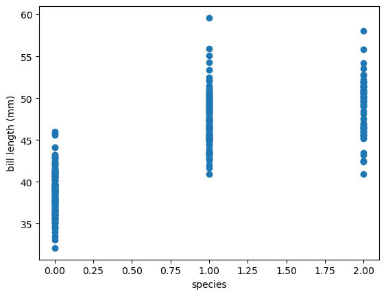
If you were to fit a straight line through \(x = 0\) and \(x = 1\), it would have some meaning: the intersections would be the average bill lengths of Adelie and Gentoo penguins, respectively. But if the fit also includes \(x = 2\), it would be meaningless, since it would be using the order of Adelie, Gentoo, and Chinstrap, as well as the equal spacing between them, as relevant for determining the \(y\) predictions.

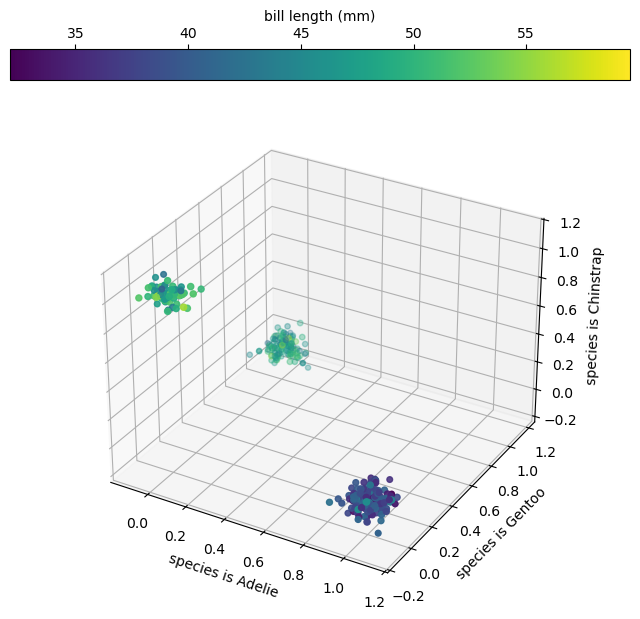
On the other hand, the one-hot encoding is difficult to visualize, but any fits through this high-dimensional space are meaningful.

fig = plt.figure(figsize=(8, 8))
ax = fig.add_subplot(projection="3d")

jitter = np.random.normal(0, 0.05, (len(categorical_1hot_df), 3))

vis = ax.scatter(
    categorical_1hot_df["species_Adelie"] + jitter[:, 0],
    categorical_1hot_df["species_Gentoo"] + jitter[:, 1],
    categorical_1hot_df["species_Chinstrap"] + jitter[:, 2],
    c=categorical_1hot_df["bill_length_mm"],   # color of points is bill length
    s=categorical_1hot_df["bill_depth_mm"],    # size of points is bill depth
)
ax.set_xlabel("species is Adelie")
ax.set_ylabel("species is Gentoo")
ax.set_zlabel("species is Chinstrap")

plt.colorbar(vis, ax=ax, label="bill length (mm)", location="top")

plt.show()

It’s also possible for all of the features and predictions in a problem to be categorical. For instance, suppose the model is given a penguin’s species and is asked to predict its probable island (so we can bring it home!).

pd.get_dummies(penguins_df.dropna()[["species", "island"]])

	species_Adelie	species_Chinstrap	species_Gentoo	island_Biscoe	island_Dream	island_Torgersen
0	True	False	False	False	False	True
1	True	False	False	False	False	True
2	True	False	False	False	False	True
4	True	False	False	False	False	True
5	True	False	False	False	False	True
...	...	...	...	...	...	...
339	False	True	False	False	True	False
340	False	True	False	False	True	False
341	False	True	False	False	True	False
342	False	True	False	False	True	False
343	False	True	False	False	True	False

333 rows × 6 columns

Here’s what we’ll use as our sample problem: given the bill length and depth, what is the penguin’s species?

fig, ax = plt.subplots()

def plot_categorical_problem(ax, xlow=29, xhigh=61, ylow=12, yhigh=22):
    df_Adelie = categorical_1hot_df[categorical_1hot_df["species_Adelie"] == 1]
    df_Gentoo = categorical_1hot_df[categorical_1hot_df["species_Gentoo"] == 1]
    df_Chinstrap = categorical_1hot_df[categorical_1hot_df["species_Chinstrap"] == 1]

    ax.scatter(df_Adelie["bill_length_mm"], df_Adelie["bill_depth_mm"], color="tab:blue", label="Adelie")
    ax.scatter(df_Gentoo["bill_length_mm"], df_Gentoo["bill_depth_mm"], color="tab:orange", label="Gentoo")
    ax.scatter(df_Chinstrap["bill_length_mm"], df_Chinstrap["bill_depth_mm"], color="tab:green", label="Chinstrap")

    ax.set_xlim(xlow, xhigh)
    ax.set_ylim(ylow, yhigh)
    ax.set_xlabel("bill length (mm)")
    ax.set_ylabel("bill depth (mm)")

    ax.legend(loc="lower left", framealpha=1)

plot_categorical_problem(ax)

plt.show()

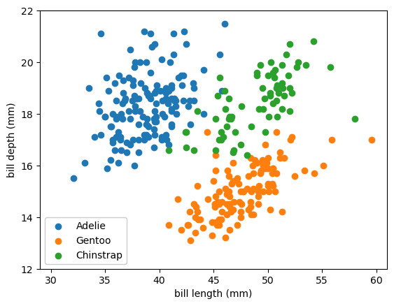
The model will be numerical, a function from bill length and depth to a 3-dimensional probability space. Probabilities have two hard constraints:

• they are all strictly bounded between \(0\) and \(1\)

• all the probabilities in a set of possibilities need to add up to \(1\).

If we define \(P_A\), \(P_G\), and \(P_C\) for the probability that a penguin is Adelie, Gentoo, or Chinstrap, respectively, then \(P_A + P_G + P_C = 1\) and all are non-negative.

One way to ensure the first constraint is to let a model predict values between \(-\infty\) and \(\infty\), then pass them through a sigmoid function:

\[p(x) = \frac{1}{1 + \exp(x)}\]

If we only had 2 categories, \(P_1\) and \(P_2\), this would be sufficient: we’d model the probability of \(P_1\) only by applying a sigmoid as the last step in our model. \(P_2\) can be inferred from \(P_1\).

But what if we have 3 categories, as in the penguin problem?

The sigmoid function has a multidimensional generalization called softmax. Given an \(n\)-dimensional vector \(\vec{x}\) with components \(x_1, x_2, \ldots, x_n\),

\[P(\vec{x})_i = \frac{\exp(x_i)}{\displaystyle \sum_j^n \exp(x_j)}\]

For any \(x_i\) between \(-\infty\) and \(\infty\), all \(0 \le P_i \le 1\) and \(\sum_i P_i = 1\). Thus, we can pass the output of any \(n\)-dimensional vector through a softmax to get probabilities.

Scikit-Learn

In keeping with the principle that a linear fit is the simplest kind of neural network, we can use Scikit-Learn’s LogisticRegression as a single-layer neural network.

from sklearn.linear_model import LogisticRegression

Scikit-Learn requires the target classes to be passed as integer labels, so we use categorical_int_df, rather than categorical_1hot_df.

categorical_features = categorical_int_df[["bill_length_mm", "bill_depth_mm"]].values
categorical_targets = categorical_int_df["species"].values

The reason we set penalty=None is (again) to stop it from applying regularization, which we’ll learn about later.

best_fit = LogisticRegression(penalty=None).fit(categorical_features, categorical_targets)

fig, ax = plt.subplots()

def plot_categorical_solution(ax, model, xlow=29, xhigh=61, ylow=12, yhigh=22):
    # compute the three probabilities for every 2D point in the background
    background_x, background_y = np.meshgrid(np.linspace(xlow, xhigh, 100), np.linspace(ylow, yhigh, 100))
    background_2d = np.column_stack([background_x.ravel(), background_y.ravel()])
    probabilities = model(background_2d)
    
    # draw contour lines where the probabilities cross the 50% threshold
    ax.contour(background_x, background_y, probabilities[:, 0].reshape(background_x.shape), [0.5])
    ax.contour(background_x, background_y, probabilities[:, 1].reshape(background_x.shape), [0.5])
    ax.contour(background_x, background_y, probabilities[:, 2].reshape(background_x.shape), [0.5])

plot_categorical_solution(ax, lambda x: best_fit.predict_proba(x))
plot_categorical_problem(ax)

plt.show()

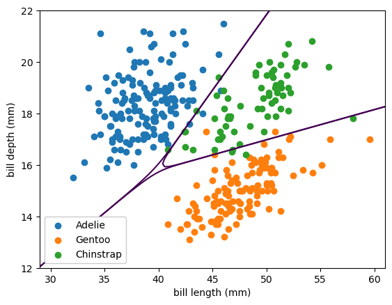
Despite being called a linear model, the best fit lines are curvy. That’s because it’s a linear fit from the 2-dimensional input space to a 3-dimensional space, which ranges from \(-\infty\) to \(\infty\) in all 3 dimensions, and then those are passed through a softmax to get 3 well-behaved probabilities.

To add a layer of ReLU functions, use Scikit-Learn’s MLPClassifier.

from sklearn.neural_network import MLPClassifier

As in the previous section, we need to scale the features to be order 1. The bill lengths and depths are 30‒60 mm and 13‒22 mm, respectively, which would be hard for the optimizer to find in small steps, starting from numbers between \(-1\) and \(1\).

But… do we need to scale the prediction targets? Why not?

def scale_features(x):
    return (x - categorical_features.mean(axis=0)) / categorical_features.std(axis=0)

categorical_features_scaled = scale_features(categorical_features)

Below, alpha=0 because we haven’t discussed regularization yet.

best_fit = MLPClassifier(
    activation="relu", hidden_layer_sizes=(5,), solver="lbfgs", max_iter=1000, alpha=0
).fit(categorical_features_scaled, categorical_targets)

fig, ax = plt.subplots()

plot_categorical_solution(ax, lambda x: best_fit.predict_proba(scale_features(x)))
plot_categorical_problem(ax)

plt.show()

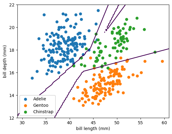
The 50% threshold lines can now be piecewise linear, because of the ReLU adaptive basis functions. (If we had chosen sigmoid/logistic, they’d be smooth curves.) These thresholds even be shrink-wrapping around individual training points, especially those that are far from the bulk of the distributions, which is less constrained.

PyTorch

Now that we’ve done regression in Scikit-Learn and PyTorch and classification in Scikit-Learn, the extension to classification in PyTorch ought to be straightforward. However, it has some tricky aspects just because of the way PyTorch works and an inherent ambiguity in what we consider part of the model.

First, the easy part: classification in PyTorch will look roughly like this:

import torch
from torch import nn, optim

# now now, just 1-dimensional features and only 2 categories
features1d = torch.tensor(categorical_features_scaled[:, 0:1], dtype=torch.float32)
targets1d = torch.tensor(categorical_targets[:, np.newaxis] == 0, dtype=torch.float32)

model = nn.Sequential(
    nn.Linear(1, 1),    # 1D → 1D linear transformation
    nn.Sigmoid(),       # sigmoid shape for probability
)

# Binary Cross Entropy as the loss function for 2 categories
loss_function = nn.BCELoss()

# a generic optimizer
optimizer = optim.Adam(model.parameters())

for epoch in range(10000):
    # almost always do this at the beginning of a step
    optimizer.zero_grad()

    # compute model predictions and loss/how bad the prediction is
    predictions = model(features1d)
    loss = loss_function(predictions, targets1d)

    # almost always do this at the end of a step
    loss.backward()
    optimizer.step()

fig, ax = plt.subplots()

ax.scatter(features1d, targets1d, marker="+", color="tab:orange", label="given targets")

model_x = np.linspace(-3, 3, 1000)
model_y = model(torch.tensor(model_x[:, np.newaxis], dtype=torch.float32)).detach().numpy()[:, 0]
ax.plot(model_x, model_y, linewidth=3, label="fitted probability")

ax.set_xlabel("scaled bill length (unitless)")
ax.set_ylabel("probability that penguin is Adelie")

ax.legend(loc="upper right")

plt.show()

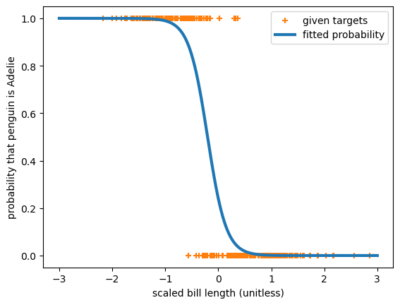
This is a 1-dimensional, linear, logistic fit of 2 categories. We can see that because the model is just a nn.Linear(1, 1) passed through a nn.Sigmoid().

The loss function is nn.BCELoss, or binary cross-entropy because when this quantity is minimized, the sigmoid approximates the probability of the 2 categories.

It has a generalization to \(n\) categories: nn.CrossEntropyLoss. When this full cross-entropy loss is minimized, the softmax approximates the probability of the \(n\) categories.

However, that nn.CrossEntropyLoss is tricky to use. First, it assumes that the model output (the predictions that you provide as its first argument) do not have the softmax applied. If you want to make any plots, you’ll need to apply the softmax, so I often create two functions, one with the softmax included, the other without.

The other tricky part is that what it computes depends on the data type of the targets (the targets that you provide as its second argument).

• If targets has dtype=torch.int64, PyTorch assumes each entry is an integer-encoded category label \(\in [0, n)\).

• If targets has dtype=torch.float32, PyTorch assumes each entry is a length-\(n\) subarray of non-negative category probabilities that add up to \(1\).

To see this, let’s create some artificial examples and pass them to the function. (This is an important debugging technique! You have to understand what your tools do!)

Here are some targets expressed as category probabilities. Since they’re targets, and therefore givens, they’ll almost always be zeros and ones—likely derived from a one-hot encoding.

targets_as_probabilities = torch.tensor([
    [1, 0, 0],
    [0, 1, 0],
    [0, 0, 1],
    [0, 1, 0],
    [1, 0, 0],
], dtype=torch.float32)

Here are the same targets expressed as category labels.

targets_as_labels = torch.argmax(targets_as_probabilities, axis=1)
targets_as_labels

tensor([0, 1, 2, 1, 0])

How do they differ? In the dtype and the rank (length of the shape tuple or torch.Size array):

targets_as_probabilities.dtype, targets_as_probabilities.shape

(torch.float32, torch.Size([5, 3]))

targets_as_labels.dtype, targets_as_labels.shape

(torch.int64, torch.Size([5]))

Here are some model predictions, such as what a model without softmax might produce. There is no constraint on the values being between \(0\) and \(1\) or adding up to \(1\).

predictions = torch.tensor([
    [100,  10,  10],
    [ -5,  20,   0],
    [2.2, -10,  50],
    [150, -10,  20],
    [0.5, 123, -10],
], dtype=torch.float32)

You’d get actual probabilities if you apply the nn.Softmax.

predictions_with_softmax = nn.Softmax(dim=1)(predictions)
predictions_with_softmax

tensor([[1.0000e+00, 8.1940e-40, 8.1940e-40],
        [1.3888e-11, 1.0000e+00, 2.0612e-09],
        [1.7407e-21, 8.7565e-27, 1.0000e+00],
        [1.0000e+00, 0.0000e+00, 0.0000e+00],
        [0.0000e+00, 1.0000e+00, 0.0000e+00]])

predictions_with_softmax.sum(axis=1)

tensor([1., 1., 1., 1., 1.])

The nn.CrossEntropyLoss takes predictions without softmax and when the second argument has floating-point type, it’s presumed to be target (given) probabilities:

nn.CrossEntropyLoss()(predictions, targets_as_probabilities)

tensor(56.5000)

When the second argument has integer type, it’s presumed to be target labels:

nn.CrossEntropyLoss()(predictions, targets_as_labels)

tensor(56.5000)

(We get the same answer because these targets_as_labels correspond to the targets_as_probabilities.)

As another PyTorch technicality, notice that most of these functions create functions (or, as another way of saying it, they’re class instances with a __call__ method, so they can be called like functions). nn.CrossEntropyLoss is not a function of predictions and targets; it returns a function of predictions and targets:

nn.CrossEntropyLoss()

CrossEntropyLoss()

(This is an object you can then call as a function with two arguments.)

In principle, targets might have probabilities between \(0\) and \(1\), depending on what’s given in the problem. If so, then you must use the targets_as_probabilities method. PyTorch’s documentation says that targets_as_labels is faster.

In the next section, you’ll do the full 2-dimensional, 3-category fit in PyTorch as an exercise.