Regularization#
There are a few ways to algorithmically reduce the complexity of a neural network, and they’re all called “regularization.” The first two take advantage of the fact that we’re already minimizing an arbitrary loss function, so they just add terms that penalize complexity in the loss function.
import numpy as np
import pandas as pd
import matplotlib.pyplot as plt
L1 and L2 regularization#
A model with fewer parameters is less complex than a model with more parameters, and forcing a parameter to take on a constant value effectively removes that parameter. For a model with \(N\) parameters \(p_i\) (\(i \in [0, N)\)),
and
are both terms that can be added to a loss function \(L(\vec{p})\) to encourage the optimizer to suppress as many parameters as it can (set them close to zero) while still fitting the training data. The coefficients \(\lambda_{L1}\) and \(\lambda_{L2}\), which you choose, determine how zealous the optimizer will be in zeroing out parameter values, relative to its other goal of fitting the training data. This goes back to the issue that the output of a loss function must be 1-dimensional to be strictly ordered, so every goal has to be given a weight relative to all other goals. (Fun fact: from your physics background, you might recognize \(R_{L1}\) and \(R_{L2}\) as Lagrange multipliers.)
In playground.tensorflow.org, this choice of regularizer and its strength, \(\lambda_{L1}\) or \(\lambda_{L2}\), are called “Regularization” and “Regularization rate.”
Forcing the absolute values of all parameters toward zero, \(R_{L1}\), and forcing the squared values of all parameters toward zero, \(R_{L2}\), have slightly different consequences. Both have been used for decades in linear regression, where they’re called Lasso and Ridge, respectively (using both is called Elastic Net):
\(R_{L1}\): (1996) Robert Tibshirani, Regression Shrinkage and Selection Via the Lasso
\(R_{L2}\): (1970) Arthur Hoerl & Robert Kennard, Ridge Regression: Biased Estimation for Nonorthogonal Problems
\(R_{L1} + R_{L2}\): (2005) Hui Zou & Trevor Hastie Regularization and variable selection via the elastic net
Scikit-Learn provides Lasso, Ridge, and ElasticNet optimizers.
from sklearn.linear_model import LinearRegression, Lasso, Ridge, ElasticNet
Suppose we have the problem from the last section, 10 data points that we’d like to fit to a polynomial.
data_x = np.linspace(0, 1, 10)
data_y = 1 + 4*data_x - 5*data_x**2 + np.random.normal(0, 0.3, 10)
Before looking at the data, we don’t know how high of a polynomial degree is appropriate. So we’ll give it too high of a degree and let regularization pull the unnecessary terms to zero.
def fit_polynomial(n, fitter):
    polynomial_features = np.hstack([data_x[:, np.newaxis]**i for i in range(n + 1)])
    best_fit = fitter.fit(polynomial_features, data_y)

    model_x = np.linspace(0, 1, 1000)
    polynomial_features = np.hstack([model_x[:, np.newaxis]**i for i in range(n + 1)])
    return model_x, best_fit.predict(polynomial_features)
fig, ax = plt.subplots()

def plot_everything(ax, n, fitter, color, ls, label):
    ax.scatter(data_x, data_y, s=200, color="white", zorder=4)
    ax.scatter(data_x, data_y, s=100, color="tab:orange", zorder=5)
    ax.plot(*fit_polynomial(n, fitter), color=color, ls=ls, linewidth=2, label=label, zorder=3)
    ax.set_xlabel("x")
    ax.set_ylabel("y")
    ax.set_ylim(data_y.min() - 0.15, data_y.max() + 0.15)

plot_everything(ax, 9, LinearRegression(fit_intercept=False), "#8a9700", "-", r"$\lambda_{L1} = 0$")
plot_everything(ax, 9, Lasso(alpha=0.00001, max_iter=1000000, fit_intercept=False), "#85b954", "--", r"$\lambda_{L1} = 0.00001$")
plot_everything(ax, 9, Lasso(alpha=0.001, max_iter=1000000, fit_intercept=False), "#85d993", ":", r"$\lambda_{L1} = 0.001$")
plot_everything(ax, 9, Lasso(alpha=0.1, max_iter=1000000, fit_intercept=False), "#51c99f", "-.", r"$\lambda_{L1} = 0.1$")
plot_everything(ax, 9, Lasso(alpha=1, max_iter=1000000, fit_intercept=False), "#00b8a9", "-", r"$\lambda_{L1} = 1$")

ax.legend(title="Lasso (L1)", loc="lower center", framealpha=1)

plt.show()
/home/runner/micromamba/envs/deep-learning-intro-for-hep/lib/python3.11/site-packages/sklearn/linear_model/_coordinate_descent.py:697: ConvergenceWarning: Objective did not converge. You might want to increase the number of iterations, check the scale of the features or consider increasing regularisation. Duality gap: 1.025e-02, tolerance: 2.136e-03
  model = cd_fast.enet_coordinate_descent(
fig, ax = plt.subplots()

plot_everything(ax, 9, LinearRegression(fit_intercept=False), "#8a9700", "-", r"$\lambda_{L2} = 0$")
plot_everything(ax, 9, Ridge(alpha=1e-14, fit_intercept=False), "#85b954", "--", r"$\lambda_{L2} = 10^{-14}$")
plot_everything(ax, 9, Ridge(alpha=1e-10, fit_intercept=False), "#85d993", ":", r"$\lambda_{L2} = 10^{-10}$")
plot_everything(ax, 9, Ridge(alpha=1e-5, fit_intercept=False), "#51c99f", "-.", r"$\lambda_{L2} = 10^{-5}$")
plot_everything(ax, 9, Ridge(alpha=1, fit_intercept=False), "#00b8a9", "-", r"$\lambda_{L2} = 1$")

ax.legend(title="Ridge (L2)", loc="lower center", framealpha=1)

plt.show()
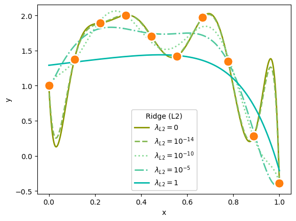
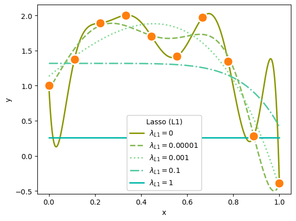
Both L1 and L2 suppress polynomial terms in proportion to the strength of \(\lambda_{L1}\) or \(\lambda_{L2}\).
In the first plot, a very strong \(\lambda_{L1} = 1\) completely zeroed out all polynomial terms except for the constant; the model effectively computed an average.
In the second plot, a very weak \(\lambda_{L2} = 10^{-14}\) is almost—but not quite—the same as a purely linear fit.
To get visible effects, I had to set \(\lambda_{L1}\) and \(\lambda_{L2}\) to very different orders of magnitude, and the Lasso (L1) regularization needed more iterations (max_iter) to converge.
(One more thing that I should point out: if you want to use this technique in a real application, use Legendre polynomials as the terms in the linear fit, rather than \(x^0\), \(x^1\), \(x^2\), etc., since Legendre polynomials are orthonormal with uniform weight on the interval \((-1, 1)\). Also, scale \((-1, 1)\) to the domain of your actual data. Notice that in this fit, the highly constrained polynomials are more constrained by the point at \(x = 1\) than any other point!)
Dissecting L1 and L2 regularization#
Let’s look at what they do in more detail on 2-dimensional fits. First, let’s make datasets in which \(y\) is a linear function of \(x_1\) and \(x_2\) at some angle.
def make_dataset(angle, n):
    x = np.random.uniform(0, 1, (n, 2))
    y = np.cos(angle) * x[:, 0] + np.sin(angle) * x[:, 1] + np.random.normal(0, 0.3, n)
    return x, y
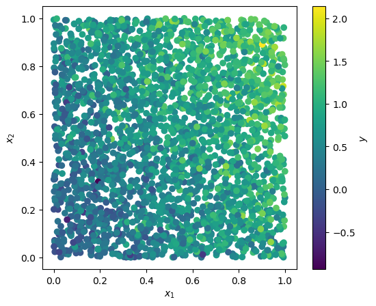
At an angle of \(\pi/6\) (30 degrees), it looks like this:
fig, ax = plt.subplots(figsize=(6, 5))

def plot_dataset(x, y):
    plt.colorbar(ax.scatter(x[:, 0], x[:, 1], c=y), label="$y$")
    ax.set_xlabel("$x_1$")
    ax.set_ylabel("$x_2$")

x, y = make_dataset(np.pi / 6, 3000)
plot_dataset(x, y)

plt.show()
Now let’s make a lot of datasets at different angles, from \(-\pi/4\) (45 degrees below the horizontal) to \(3\pi/4\) (45 degrees beyond the vertical), and fit each one with an unconstrained linear fit, Lasso (L1), and Ridge (L2) regularization.
def fitted_parameters(fitter, x, y):
    return fitter.fit(x, y).coef_
fig, ax = plt.subplots(figsize=(5, 5))

linear_parameters = np.empty((100, 2))
lasso_parameters = np.empty((100, 2))
ridge_parameters = np.empty((100, 2))

for i, angle in enumerate(np.linspace(-np.pi/4, 3*np.pi/4, 100)):
    x, y = make_dataset(angle, 10000)
    linear_parameters[i] = fitted_parameters(LinearRegression(fit_intercept=False), x, y)
    lasso_parameters[i] = fitted_parameters(Lasso(alpha=0.1, fit_intercept=False), x, y)
    ridge_parameters[i] = fitted_parameters(Ridge(alpha=1000, fit_intercept=False), x, y)

ax.scatter(linear_parameters[:, 0], linear_parameters[:, 1], label="Unconstrained linear fits")
ax.scatter(lasso_parameters[:, 0], lasso_parameters[:, 1], label=r"Lasso (L1) with $\lambda_{L1} = 0.1$")
ax.scatter(ridge_parameters[:, 0], ridge_parameters[:, 1], label=r"Ridge (L2) with $\lambda_{L2} = 1000$")

ax.axvline(0, color="gray", ls=":", zorder=-1)
ax.axhline(0, color="gray", ls=":", zorder=-1)

ax.set_xlim(-0.8, 1.1)
ax.set_ylim(-0.8, 1.1)
ax.set_xlabel("slope of $x_1$")
ax.set_ylabel("slope of $x_2$")

ax.legend(loc="lower left", framealpha=1)

plt.show()
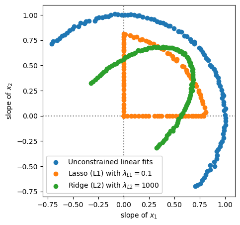
The unconstrained linear fits make a semicircle in the two fitted parameters, slope of \(x_1\) and slope of \(x_2\), because that’s what the datasets do.
Lasso (L1) regularization either suppresses both parameters or completely zeros one of them out.
Ridge (L2) regularization is always smooth: it suppresses both parameters.
(The first quadrant, in which the true slopes of \(x_1\) and \(x_2\) are both positive, is different from the second and fourth quadrants, in which one is negative, because in the second and fourth quadrants both parameters need to have large magnitudes to cancel each other, to fit the data appropriately.)
Bottom line: Lasso (L1) regularization has sharp, discrete effects on the parameters, and in particular tends to lock them at zero if they’re not necessary for fitting the training data. This is why a strong \(\lambda_{L1}\) reduced the polynomial fit to a single-term constant. Ridge (L2) regularization produces smooth models.
Realistic use of regularization (linear)#
The two examples above are synthetic, intended to provide intuition about what L1 and L2 regularization do and how they work. How would they actually be used for a real problem?
Let’s start with the Boston House Prices dataset.
boston_prices_df = pd.read_csv(
    "data/boston-house-prices.csv", sep="\s+", header=None,
    names=["CRIM", "ZN", "INDUS", "CHAS", "NOX", "RM", "AGE", "DIS", "RAD", "TAX", "PTRATIO", "B", "LSTAT", "MEDV"],
)

# Pre-normalize the data so we can ignore that part of modeling
boston_prices_df = (boston_prices_df - boston_prices_df.mean()) / boston_prices_df.std()

features = boston_prices_df.drop(columns=["MEDV"])
targets = boston_prices_df["MEDV"]
Remember that the 13 features of this dataset quantify a variety of things, all of which seem like they might have some effect on housing prices (or perhaps they were included to demonstrate/discover a null effect).
CRIM: per capita crime rate per town
ZN: proportion of residental land zoned for lots over 25,000 square feet
INDUS: proportion of non-retail business acres per town
CHAS: adjacency to the Charles River (a boolean variable)
NOX: nitric oxides concentration (parts per 10 million)
RM: average number of rooms per dwelling
AGE: proportion of owner-occupied units built before 1940
DIS: weighted distances to 5 Boston employment centers
RAD: index of accessiblity to radial highways
TAX: full-value property-tax rate per $10,000
PTRATIO: pupil-teacher ratio by town
B: \(1000(b - 0.63)^2\) where \(b\) is the proportion of Black residents
LSTAT: % lower status by population
This is a “throw everything into the model and see what’s relevant” kind of analysis. If the dataset is large enough, unimportant features should have a slope that is statistically consistent with zero, but this dataset only has 506 rows (towns near Boston). Rather than a null hypothesis analysis, let’s find out which features are the most disposable by fitting it with Lasso (L1) regularization, to see which features it zeros out first.
def lasso_fit_with(alpha):
    best_fit = Lasso(alpha=alpha).fit(features.values, targets.values)
    return features.columns[best_fit.coef_ != 0].tolist()

print(lasso_fit_with(0.0001))
print(lasso_fit_with(0.015))
print(lasso_fit_with(0.02))
print(lasso_fit_with(0.023))
print(lasso_fit_with(0.03))
print(lasso_fit_with(0.05))
print(lasso_fit_with(0.06))
print(lasso_fit_with(0.07))
print(lasso_fit_with(0.1))
print(lasso_fit_with(0.13))
print(lasso_fit_with(0.3))
print(lasso_fit_with(0.6))
print(lasso_fit_with(0.7))
['CRIM', 'ZN', 'INDUS', 'CHAS', 'NOX', 'RM', 'AGE', 'DIS', 'RAD', 'TAX', 'PTRATIO', 'B', 'LSTAT']
['CRIM', 'ZN', 'INDUS', 'CHAS', 'NOX', 'RM', 'DIS', 'RAD', 'TAX', 'PTRATIO', 'B', 'LSTAT']
['CRIM', 'ZN', 'INDUS', 'CHAS', 'NOX', 'RM', 'DIS', 'RAD', 'PTRATIO', 'B', 'LSTAT']
['CRIM', 'ZN', 'INDUS', 'CHAS', 'NOX', 'RM', 'DIS', 'PTRATIO', 'B', 'LSTAT']
['CRIM', 'ZN', 'CHAS', 'NOX', 'RM', 'DIS', 'PTRATIO', 'B', 'LSTAT']
['CRIM', 'CHAS', 'NOX', 'RM', 'DIS', 'PTRATIO', 'B', 'LSTAT']
['CRIM', 'CHAS', 'RM', 'DIS', 'PTRATIO', 'B', 'LSTAT']
['CRIM', 'CHAS', 'RM', 'PTRATIO', 'B', 'LSTAT']
['CHAS', 'RM', 'PTRATIO', 'B', 'LSTAT']
['RM', 'PTRATIO', 'B', 'LSTAT']
['RM', 'PTRATIO', 'LSTAT']
['RM', 'LSTAT']
['LSTAT']
Realistic use of regularization (ML)#
Neural networks also construct features, internally as combinations of hidden layer components. If you don’t know what combinations of input variables are relevant, include enough hidden layers with enough components and the fit will construct what it needs. However, it will also construct too much and overfit the training data.
So let’s apply Ridge (L2) regularization to an overparameterized neural network and see what happens to the loss and parameters.
import torch
from torch import nn, optim
def nn_with_l2(alpha, num_hidden_layers=100, num_epochs=1000, manual_seed=12345):
    torch.manual_seed(manual_seed)

    features_tensor = torch.tensor(features.values, dtype=torch.float32)
    targets_tensor = torch.tensor(targets.values[:, np.newaxis], dtype=torch.float32)

    model = nn.Sequential(
        nn.Linear(13, num_hidden_layers),
        nn.ReLU(),
        nn.Linear(num_hidden_layers, 1),
    )

    loss_function = nn.MSELoss()
    optimizer = optim.Adam(model.parameters())

    loss_vs_epoch = []

    for epoch in range(num_epochs):
        optimizer.zero_grad()

        unconstrained_loss = loss_function(model(features_tensor), targets_tensor)

        # as usual, PyTorch makes you calculate it yourself
        l2_term = sum(p.pow(2).sum() for p in model.parameters())

        loss = unconstrained_loss + alpha * l2_term
        loss_vs_epoch.append(loss.item())

        loss.backward()
        optimizer.step()

    return model, loss_vs_epoch
fig, ax = plt.subplots()

model_unconstrained, loss_vs_epoch = nn_with_l2(0)
ax.plot(range(1, len(loss_vs_epoch) + 1), loss_vs_epoch, label=r"$\lambda_{L2} = 0$")
ax.axhline(loss_vs_epoch[-1], color="tab:blue", ls=":")

model_01, loss_vs_epoch = nn_with_l2(0.1)
ax.plot(range(1, len(loss_vs_epoch) + 1), loss_vs_epoch, label=r"$\lambda_{L2} = 0.1$")
ax.axhline(loss_vs_epoch[-1], color="tab:orange", ls=":")

ax.set_ylim(0, 1.1)
ax.set_xlabel("epoch number")
ax.set_ylabel("loss")

ax.legend(loc="upper right")

plt.show()
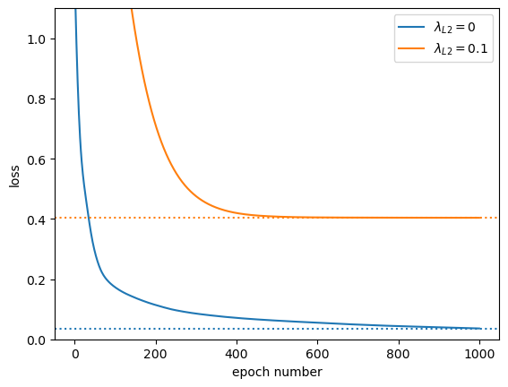
The loss-versus-epoch is always higher for \(\lambda_{L2} = 0.1\) because we’ve added an extra term. But also notice how it flattens out after 400 epochs; it’s not getting arbitrarily better by overfitting the data.
fig, ax = plt.subplots()

ax.hist(np.concatenate(
    [x.detach().numpy().ravel() for x in model_unconstrained.parameters()]
), bins=100, range=(-0.5, 0.5), histtype="step", label=r"$\lambda_{L2} = 0$")
ax.hist(np.concatenate(
    [x.detach().numpy().ravel() for x in model_01.parameters()]
), bins=100, range=(-0.5, 0.5), histtype="step", label=r"$\lambda_{L2} = 0.1$")

ax.set_xlabel("model parameter values")

ax.legend(loc="upper right")

plt.show()
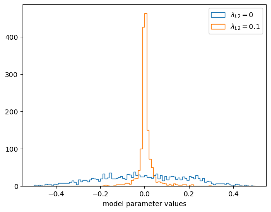
Most of the model parameters are closer to zero because of the Ridge (L2) constraint.
Dropout regularization#
If the problem we’re trying to solve is that our neural network has too many parameters, why not just drop them? Randomly zeroing out parameters and letting the optimization “heal” the model around the missing parameters is often effective (ref).
The way that you apply this technique is fundamentally different from L1 and L2 regularization: it’s not a term in the loss function. PyTorch provides a nn.Dropout layer that you can insert after every activation function in your model.
dropout = nn.Dropout(p=0.8)

def print_effect_of_dropout(vector_entering_layer):
    vector_after_dropout = dropout(vector_entering_layer)

    print("   * means this hidden layer component is included\n")
    print("  ", "".join(f"{i*10:10d}" for i in range(1, 9)))
    for i, row in enumerate(vector_after_dropout):
        print(f"{i + 1:2d}", "".join(" " if x == 0 else "*" for x in row))
For 10 training events, its effect on 80 components of a hidden layer looks like this:
dropout.train()
print_effect_of_dropout(torch.ones((10, 80)))
   * means this hidden layer component is included

           10        20        30        40        50        60        70        80
 1          ***   **    *  *        *                    **  *                *   *
 2               ** *   *  *        **                        **  *  *  *       **
 3  *        *       *    **             **     ***   *                *  ** ***
 4     * *  *  *       *  * **    * *            *  *     *** * *   **  **   *
 5        ***      *   **      * *   *        *    *   *   * *    * *          *
 6          ***              *   *               **   *  *    * * *  * *
 7           *        **    **       *     **            *   **      *      *    *
 8 ** *    *      *  ***   *     **      *   *       *      *      *  *    * **
 9  * *  **    *                 *  *    *                    * * **         *
10  *  ** *           *   *       * *        **  *    **      * *    **
After the model has been trained, we want all of the parameters to be turned back on. To switch between these modes, PyTorch provides nn.Module.train and nn.Module.eval:
dropout.eval()
print_effect_of_dropout(torch.ones((10, 80)))
   * means this hidden layer component is included

           10        20        30        40        50        60        70        80
 1 ********************************************************************************
 2 ********************************************************************************
 3 ********************************************************************************
 4 ********************************************************************************
 5 ********************************************************************************
 6 ********************************************************************************
 7 ********************************************************************************
 8 ********************************************************************************
 9 ********************************************************************************
10 ********************************************************************************
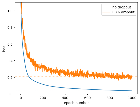
By randomly dropping parameters during training, the parameters are forced to be able to work independently: random subsets are individually optimized to fit the function. When we’re ready to use the model for prediction, the effect of all of the random subsets are added together by turning them all on. Thus, a neural network with dropout is a kind of ensemble model: it avoids overfitting by independently training submodels and then averaging their predictions.
Let’s see what it does for the Boston House Price dataset:
torch.manual_seed(12345)

model = nn.Sequential(
    nn.Linear(13, 100),
    nn.ReLU(),
    nn.Linear(100, 1),
)
torch.manual_seed(12345)

model_with_dropout = nn.Sequential(
    nn.Linear(13, 100),
    nn.ReLU(),
    nn.Dropout(p=0.8),    # 80% of vector components will be zeroed out
    nn.Linear(100, 1),
)
def fit_nn(model, num_epochs=1000):
    features_tensor = torch.tensor(features.values, dtype=torch.float32)
    targets_tensor = torch.tensor(targets.values[:, np.newaxis], dtype=torch.float32)

    loss_function = nn.MSELoss()
    optimizer = optim.Adam(model.parameters())

    loss_vs_epoch = []

    # set the model for its training phase
    model.train()

    for epoch in range(num_epochs):
        optimizer.zero_grad()

        loss = loss_function(model(features_tensor), targets_tensor)
        loss_vs_epoch.append(loss.item())

        loss.backward()
        optimizer.step()

    # set the model for its evaluation phase
    model.eval()

    return loss_vs_epoch
fig, ax = plt.subplots()

loss_vs_epoch = fit_nn(model)
ax.plot(range(1, len(loss_vs_epoch) + 1), loss_vs_epoch, label="no dropout")
ax.axhline(loss_vs_epoch[-1], color="tab:blue", ls=":")

loss_vs_epoch = fit_nn(model_with_dropout)
ax.plot(range(1, len(loss_vs_epoch) + 1), loss_vs_epoch, label="80% dropout")
ax.axhline(loss_vs_epoch[-1], color="tab:orange", ls=":")

ax.set_ylim(0, 1.1)
ax.set_xlabel("epoch number")
ax.set_ylabel("loss")

ax.legend(loc="upper right")

plt.show()
fig, ax = plt.subplots()

ax.hist(np.concatenate(
    [x.detach().numpy().ravel() for x in model.parameters()]
), bins=100, range=(-0.5, 0.5), histtype="step", label="no dropout")
ax.hist(np.concatenate(
    [x.detach().numpy().ravel() for x in model_with_dropout.parameters()]
), bins=100, range=(-0.5, 0.5), histtype="step", label="80% dropout")

ax.set_xlabel("model parameter values")

ax.legend(loc="upper right")

plt.show()
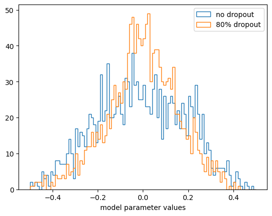
Unlike L1 and L2 regularization, the parameter values are not much smaller than without dropout (but they’re much more redundant and don’t try to optimize every point in the training dataset).
Early stopping#
In an upcoming section, we’ll cover hyperparameter optimization and validation, in which we’ll divide a dataset into a subset for training and another (one or two) for tests. The value of the loss function on the training dataset can get arbitrarily small as the model overfits, but the value of the loss function on data not used in training is a good indication of how well the model generalizes.
Let’s see what the training and test loss look like for an overfitted model. Below, we’re using Datasets and DataLoaders for convenience, because they work with PyTorch’s random_split function.
from torch.utils.data import TensorDataset, DataLoader, random_split
features_tensor = torch.tensor(features.values, dtype=torch.float32)
targets_tensor = torch.tensor(targets.values[:, np.newaxis], dtype=torch.float32)

dataset = TensorDataset(features_tensor, targets_tensor)

train_size = int(np.floor(0.8 * len(dataset)))
test_size = len(dataset) - train_size
train_dataset, test_dataset = random_split(dataset, [train_size, test_size])

train_loader = DataLoader(train_dataset, batch_size=len(train_dataset))   # only 1 batch
test_loader = DataLoader(test_dataset, batch_size=len(test_dataset))      # only 1 batch
model = nn.Sequential(
    nn.Linear(13, 100),
    nn.ReLU(),
    nn.Linear(100, 1),
)

loss_function = nn.MSELoss()
optimizer = optim.Adam(model.parameters())

train_loss = []
test_loss = []

for epoch in range(1000):
    for batch_features, batch_targets in train_loader:
        optimizer.zero_grad()

        predictions = model(batch_features)
        loss = loss_function(predictions, batch_targets)

        train_loss.append(loss.item())

        loss.backward()
        optimizer.step()

    for batch_features, batch_targets in test_loader:
        predictions = model(batch_features)
        loss = loss_function(predictions, batch_targets)

        test_loss.append(loss.item())
fig, ax = plt.subplots()

ax.plot(range(1, len(train_loss) + 1), train_loss, label="in train dataset")
ax.plot(range(1, len(test_loss) + 1), test_loss, color="tab:blue", ls=":", label="in test dataset")

ax.set_ylim(0, min(max(train_loss), max(test_loss)))
ax.set_xlabel("epoch number")
ax.set_ylabel("loss")

ax.legend(loc="upper right")

plt.show()
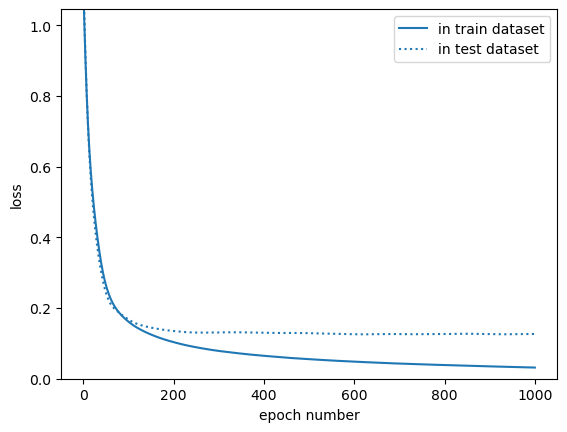
This is a diagnostic to identify overfitting: the loss calculated on the training dataset gets better than the loss calculated on the test dataset after about epoch 200 or so. You can use this distinction to determine an optimal \(\lambda_{L1}\) or \(\lambda_{L2}\) in L1 or L2 regularization, or an optimal p fraction of hidden layer components to zero out to get the training loss to level out where the test loss levels out.
Or you can be lazy (or in a hurry) and just stop training at epoch 200. This is called “early stopping,” and it is a widely used technique to prevent overfitting. It’s fragile: the epoch number in which training loss overtakes testing loss would be different for every model, and it would change when any other hyperparameters change, but it’s generally true that hyperparameters depend on each other.

