Regression in PyTorch

This and the next section introduce PyTorch so that we can use it for the remainder of the course. Whereas Scikit-Learn gives you a function for just about every type of machine learning model, PyTorch gives you the pieces and expects you to build it yourself. (The JAX library is even more extreme in providing only the fundamental pieces. PyTorch’s level of abstraction is between JAX and Scikit-Learn.)

I’ll use the two types of problems we’ve seen so far—regression and classification—to show Scikit-Learn and PyTorch side-by-side. First, though, let’s get a dataset that will provide us with realistic regression and classification problems.

import numpy as np
import pandas as pd
import matplotlib.pyplot as plt

Penguins!

This is my new favorite dataset: basic measurements on 3 species of penguins. You can get the data as a CSV file from the original source or from this project’s GitHub: deep-learning-intro-for-hep/data/penguins.csv.

Replace data/penguins.csv with the file path where you saved the file after downloading it.

penguins_df = pd.read_csv("data/penguins.csv")
penguins_df

	species	island	bill_length_mm	bill_depth_mm	flipper_length_mm	body_mass_g	sex	year
0	Adelie	Torgersen	39.1	18.7	181.0	3750.0	male	2007
1	Adelie	Torgersen	39.5	17.4	186.0	3800.0	female	2007
2	Adelie	Torgersen	40.3	18.0	195.0	3250.0	female	2007
3	Adelie	Torgersen	NaN	NaN	NaN	NaN	NaN	2007
4	Adelie	Torgersen	36.7	19.3	193.0	3450.0	female	2007
...	...	...	...	...	...	...	...	...
339	Chinstrap	Dream	55.8	19.8	207.0	4000.0	male	2009
340	Chinstrap	Dream	43.5	18.1	202.0	3400.0	female	2009
341	Chinstrap	Dream	49.6	18.2	193.0	3775.0	male	2009
342	Chinstrap	Dream	50.8	19.0	210.0	4100.0	male	2009
343	Chinstrap	Dream	50.2	18.7	198.0	3775.0	female	2009

344 rows × 8 columns

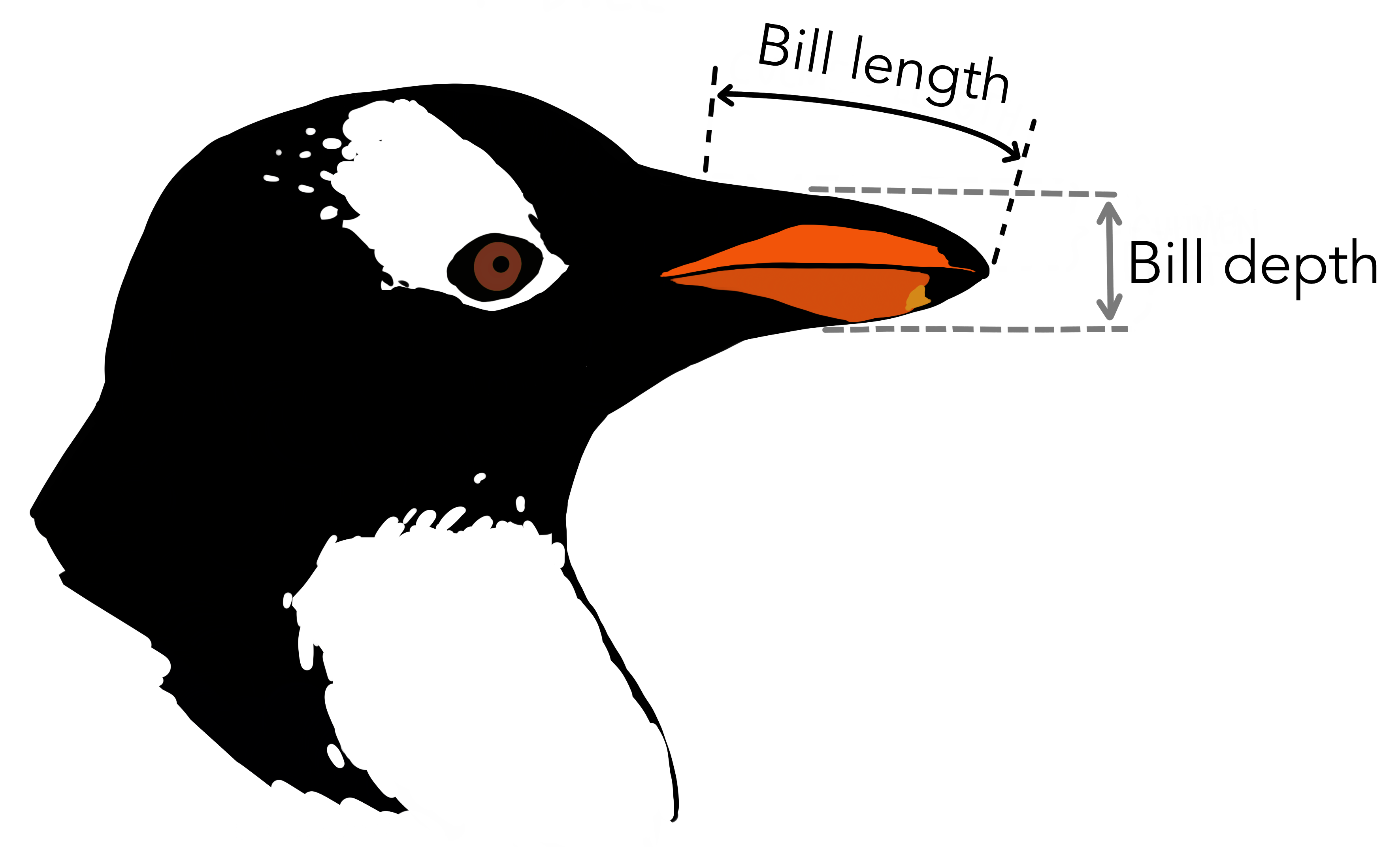
This dataset has numerical features, such as bill_length_mm, bill_depth_mm, flipper_length_mm, body_mass_g and year of data-taking, and it has categorical features like species, island, and sex. Some of the measurements are missing (NaN), but we’ll ignore them with pd.DataFrame.dropna.

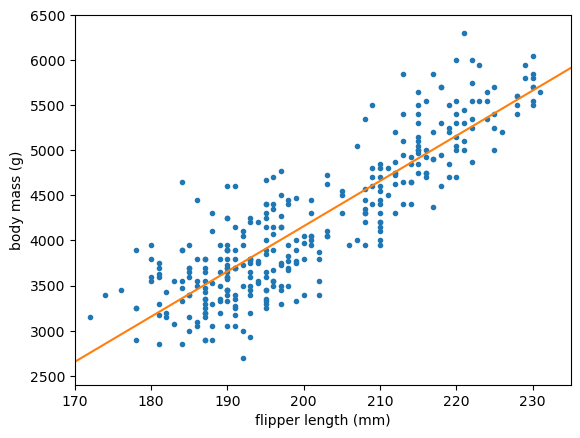
For our regression problem, let’s ask, “Given a flipper length (mm), what is the penguin’s most likely body mass (g)?”

regression_features, regression_targets = penguins_df.dropna()[["flipper_length_mm", "body_mass_g"]].values.T

fig, ax = plt.subplots()

def plot_regression_problem(ax, xlow=170, xhigh=235, ylow=2400, yhigh=6500):
    ax.scatter(regression_features, regression_targets, marker=".")
    ax.set_xlim(xlow, xhigh)
    ax.set_ylim(ylow, yhigh)
    ax.set_xlabel("flipper length (mm)")
    ax.set_ylabel("body mass (g)")

plot_regression_problem(ax)

plt.show()

Scikit-Learn

In keeping with the principle that a linear fit is the simplest kind of neural network, we can use Scikit-Learn’s LinearRegression as a single-layer, no-activation neural network:

from sklearn.linear_model import LinearRegression

best_fit = LinearRegression().fit(regression_features[:, np.newaxis], regression_targets)

fig, ax = plt.subplots()

def plot_regression_solution(ax, model, xlow=170, xhigh=235):
    model_x = np.linspace(xlow, xhigh, 1000)
    model_y = model(model_x)
    ax.plot(model_x, model_y, color="tab:orange")

plot_regression_solution(ax, lambda x: best_fit.predict(x[:, np.newaxis]))
plot_regression_problem(ax)

plt.show()

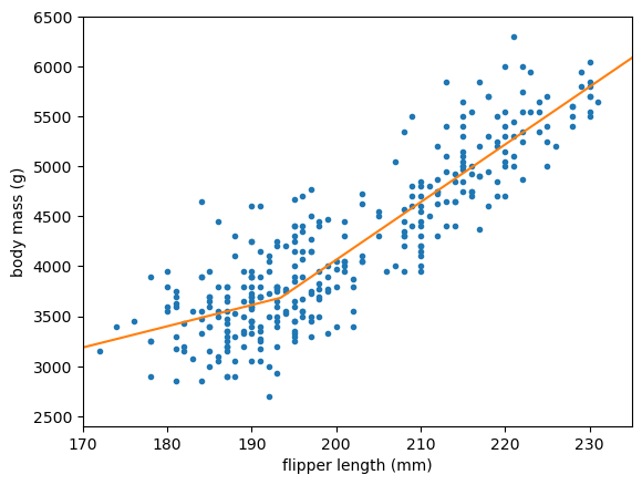
Next, let’s add a layer of ReLU functions using Scikit-Learn’s MLPRegressor. The reason we set alpha=0 is because its regularization is not off by default, and we haven’t talked about regularization yet. The solver="lbfgs" picks a more robust optimization method for this low-dimension problem.

from sklearn.neural_network import MLPRegressor

best_fit = MLPRegressor(
    activation="relu", hidden_layer_sizes=(5,), solver="lbfgs", max_iter=1000, alpha=0, random_state=123
).fit(regression_features[:, np.newaxis], regression_targets)

fig, ax = plt.subplots()

plot_regression_solution(ax, lambda x: best_fit.predict(x[:, np.newaxis]))
plot_regression_problem(ax)

plt.show()

PyTorch

Now let’s do the same in PyTorch. First, the linear model: nn.Linear(1, 1) means a linear transformation from a 1-dimensional space to a 1-dimensional space.

import torch
from torch import nn, optim

model = nn.Linear(1, 1)
model

Linear(in_features=1, out_features=1, bias=True)

A model has parameters that the optimizer will vary in the fit. When you create a model, they’re already given random values (one slope and one intercept, in this case). requires_grad refers to the fact that the derivatives of the parameters are also tracked, for the optimization methods that use derivatives.

list(model.parameters())

[Parameter containing:
 tensor([[-0.4867]], requires_grad=True),
 Parameter containing:
 tensor([-0.6008], requires_grad=True)]

We can’t pass NumPy arrays directly into PyTorch—they have to be converted into PyTorch’s own array type (which can reside on CPU or GPU), called Tensor.

PyTorch’s functions are very sensitive to the exact data types of these tensors: the difference between integers and floating-point can make PyTorch run a different algorithm! For floating-point numbers, PyTorch prefers 32-bit.

tensor_features = torch.tensor(regression_features[:, np.newaxis], dtype=torch.float32)
tensor_targets = torch.tensor(regression_targets[:, np.newaxis], dtype=torch.float32)

Now we need to say how we’re going to train the model.

• What will the loss function be? For a regression problem, it would usually be \(\chi^2\), or mean squared error: nn.MSELoss

• Which optimizer should we choose? (This is the equivalent of solver="lbfgs" in Scikit-Learn.) We’ll talk more about these later, and the right choice will usually be nn.Adam, but not for this linear problem. For now, we’ll use nn.Rprop.

The optimizer has access to the model’s parameters, and it will modify them in-place.

loss_function = nn.MSELoss()

optimizer = optim.Rprop(model.parameters())

To actually train the model, you have to write your own loop! It’s more verbose, but you get to control what happens and debug it.

One step in optimization is called an “epoch.” In Scikit-Learn, we set max_iter=1000 to get 1000 epochs. In PyTorch, we write,

for epoch in range(1000):
    # tell the optimizer to begin an optimization step
    optimizer.zero_grad()

    # use the model as a prediction function: features → prediction
    predictions = model(tensor_features)

    # compute the loss (χ²) between these predictions and the intended targets
    loss = loss_function(predictions, tensor_targets)

    # tell the loss function and optimizer to end an optimization step
    loss.backward()
    optimizer.step()

The optimizer.zero_grad(), loss.backward(), and optimizer.step() calls change the state of the optimizer and the model parameters, but you can think of them just as the beginning and end of an optimization step.

There are other state-changing functions, like model.train() (to tell it we’re going to start training) and model.eval() (to tell it we’re going to start using it for inference), but we won’t be using any of the features that depend on the variables that these set.

Now, to draw a plot with this model, we’ll have to turn the NumPy x positions into a Tensor, run it through the model, and then convert the model’s output back into a NumPy array. The output has derivatives as well as values, so those will need to be detached.

• NumPy x to Torch: torch.tensor(x, dtype=torch.float32) (or other dtype)

• Torch y to NumPy: y.detach().numpy()

fig, ax = plt.subplots()

def numpy_model(x):
    tensor_x = torch.tensor(x[:, np.newaxis], dtype=torch.float32)
    return model(tensor_x).detach().numpy()

plot_regression_solution(ax, numpy_model)
plot_regression_problem(ax)

plt.show()

A layered neural network in PyTorch is usually represented by a class, such as this:

class NeuralNetworkWithReLU(nn.Module):
    def __init__(self, hidden_layer_size):
        super().__init__()   # let PyTorch do its initialization first

        self.step1 = nn.Linear(1, hidden_layer_size)  # 1D input → 5D
        self.step2 = nn.ReLU()                        # 5D ReLU
        self.step3 = nn.Linear(hidden_layer_size, 1)  # 5D → 1D output

    def forward(self, x):
        return self.step3(self.step2(self.step1(x)))

model = NeuralNetworkWithReLU(5)
model

NeuralNetworkWithReLU(
  (step1): Linear(in_features=1, out_features=5, bias=True)
  (step2): ReLU()
  (step3): Linear(in_features=5, out_features=1, bias=True)
)

list(model.parameters())

[Parameter containing:
 tensor([[ 0.7793],
         [ 0.3205],
         [-0.6950],
         [ 0.6524],
         [ 0.5121]], requires_grad=True),
 Parameter containing:
 tensor([-0.9203, -0.7256,  0.4993, -0.6035,  0.1182], requires_grad=True),
 Parameter containing:
 tensor([[ 0.1193, -0.1820,  0.2219,  0.3191,  0.2483]], requires_grad=True),
 Parameter containing:
 tensor([-0.2744], requires_grad=True)]

You can initialize it with as many sub-models as you want and then implement what they do to features x in the forward method.

However, I like nn.Sequential better for models that are simple sequences of layers.

model = nn.Sequential(
    nn.Linear(1, 5),
    nn.ReLU(),
    nn.Linear(5, 1),
)
model

Sequential(
  (0): Linear(in_features=1, out_features=5, bias=True)
  (1): ReLU()
  (2): Linear(in_features=5, out_features=1, bias=True)
)

list(model.parameters())

[Parameter containing:
 tensor([[-0.9063],
         [ 0.5515],
         [ 0.5911],
         [-0.1539],
         [-0.4317]], requires_grad=True),
 Parameter containing:
 tensor([-0.7952, -0.2501, -0.7541, -0.1626, -0.4663], requires_grad=True),
 Parameter containing:
 tensor([[ 0.0679,  0.0881,  0.4344, -0.3645, -0.1089]], requires_grad=True),
 Parameter containing:
 tensor([-0.4191], requires_grad=True)]

Let’s fit this one the same way we fit the single-layer model:

loss_function = nn.MSELoss()
optimizer = optim.Rprop(model.parameters())

for epoch in range(1000):
    # tell the optimizer to begin an optimization step
    optimizer.zero_grad()

    # use the model as a prediction function: features → prediction
    predictions = model(tensor_features)

    # compute the loss (χ²) between these predictions and the intended targets
    loss = loss_function(predictions, tensor_targets)

    # tell the loss function and optimizer to end an optimization step
    loss.backward()
    optimizer.step()

fig, ax = plt.subplots()

plot_regression_solution(ax, numpy_model)
plot_regression_problem(ax)

plt.show()

Chances are, you don’t see any evidence of the ReLU and the above is just a straight line.

Scroll back up to the initial model parameters. Then, look at them after the fit:

list(model.parameters())

[Parameter containing:
 tensor([[-0.9063],
         [ 3.6961],
         [ 3.7357],
         [-0.1539],
         [-0.4317]], requires_grad=True),
 Parameter containing:
 tensor([-7.9516e-01, -4.0486e+02, -4.0536e+02, -1.6257e-01, -4.6626e-01],
        requires_grad=True),
 Parameter containing:
 tensor([[ 0.0679,  6.5800,  6.9155, -0.3645, -0.1089]], requires_grad=True),
 Parameter containing:
 tensor([-405.0275], requires_grad=True)]

Initially, the model parameters are all random numbers between \(-1\) and \(1\). After fitting, some of the parameters are in the few-hundred range.

Now look at the \(x\) and \(y\) ranges on the plot: flipper lengths are hundreds of millimeters and body masses are thousands of grams. The optimizer had to gradually step values of order 1 up to values of order 100‒1000, and it took small steps to avoid jumping over the solution. In the end, the optimizer found a reasonably good fit by scaling just a few parameters up and effectively performed a purely linear fit.

We should have scaled the inputs and outputs so that the values the fitter sees are all of order 1. This is something that PyTorch assumes you will do.

In many applications, I’ve seen people scale the data independently of the model. However, I’d like to make the scaling a part of the model, so that it’s easier to keep track of when it’s been applied and when it hasn’t. We could add a nn.Linear(1, 1) to multiply and shift by two parameters, but the optimizer would again have problems with a parameter that needs to be very large. Instead, I’ll use PyTorch’s nn.Module.register_buffer to add a fixed, untunable constant to the model (which it would save if it saves the model to a file).

class AddConstant(nn.Module):
    def __init__(self, constant):
        super().__init__()   # let PyTorch do its initialization first

        self.register_buffer("constant", torch.tensor([constant], dtype=torch.float32))

    def __repr__(self):
        return f"{type(self).__name__}({self.constant.item():g})"

    def forward(self, x):
        return x + self.constant

class MultiplyByConstant(nn.Module):
    def __init__(self, constant):
        super().__init__()   # let PyTorch do its initialization first

        self.register_buffer("constant", torch.tensor([constant], dtype=torch.float32))

    def __repr__(self):
        return f"{type(self).__name__}({self.constant.item():g})"

    def forward(self, x):
        return x * self.constant

Now we can build this into the model.

model = nn.Sequential(
    AddConstant(-200),         # shift the mean to 0
    MultiplyByConstant(1/10),  # scale the variance to 1
    nn.Linear(1, 5),
    nn.ReLU(),
    nn.Linear(5, 1),
    MultiplyByConstant(800),   # scale the variance to 800
    AddConstant(4200),         # shift the mean to 4200
)
model

Sequential(
  (0): AddConstant(-200)
  (1): MultiplyByConstant(0.1)
  (2): Linear(in_features=1, out_features=5, bias=True)
  (3): ReLU()
  (4): Linear(in_features=5, out_features=1, bias=True)
  (5): MultiplyByConstant(800)
  (6): AddConstant(4200)
)

list(model.parameters())

[Parameter containing:
 tensor([[ 0.2568],
         [ 0.1571],
         [-0.3227],
         [-0.4435],
         [ 0.6164]], requires_grad=True),
 Parameter containing:
 tensor([ 0.8002,  0.4720, -0.9141, -0.1511,  0.3304], requires_grad=True),
 Parameter containing:
 tensor([[-0.0933,  0.2927, -0.0949, -0.3349, -0.1222]], requires_grad=True),
 Parameter containing:
 tensor([-0.2533], requires_grad=True)]

Even in its untrained state, the model will return values of the right order of magnitude.

model(200)

tensor([4015.9004], grad_fn=<AddBackward0>)

loss_function = nn.MSELoss()
optimizer = optim.Rprop(model.parameters())

for epoch in range(1000):
    # tell the optimizer to begin an optimization step
    optimizer.zero_grad()

    # use the model as a prediction function: features → prediction
    predictions = model(tensor_features)

    # compute the loss (χ²) between these predictions and the intended targets
    loss = loss_function(predictions, tensor_targets)

    # tell the loss function and optimizer to end an optimization step
    loss.backward()
    optimizer.step()

fig, ax = plt.subplots()

plot_regression_solution(ax, numpy_model)
plot_regression_problem(ax)

plt.show()

This time, we see the effect of the ReLU steps because the data and the model parameters have the same order of magnitude.

Conclusion

I think this illustrates an important point about working with neural networks: you cannot treat them as black boxes—you have to understand the internal parts to figure out why it is or isn’t fitting the way you want it to. Nothing told us that the ReLU parameters were effectively being ignored because the data were at the wrong scale. We had to step through the pieces to find that out.

Hand-written code, called “craftsmanship” in the Overview, is generally designed to be more compartmentalized than this. If you’re coming from a programming background, this is something to look out for! Andrej Karpathy’s excellent recipe for training neural networks starts with the warning that neural network training is a “leaky abstraction,” which is to say, you have to understand its inner workings to use it effectively—more so than other software products.

That may be why PyTorch is so popular: it forces you to look at the individual pieces, rather than maintaining the illusion that pressing a fit button will give you what you want.

Next, we’ll see how to use it for classification problems.