Epochs and mini-batches#
Unlike Minuit and Scikit-Learn, PyTorch makes you write the for loop that iterates over optimization steps. Thus, the engine is “open” in the sense that you can directly modify how optimization works.
For instance, Minuit and Scikit-Learn iterate until they detect that the parameters \(\vec{p}_i\) or loss function value \(L(\vec{p}_i)\) isn’t moving much from step \(i\) to step \(i + 1\). If you want PyTorch to do the same thing, you’d have to write it:
last_loss = None

while last_loss is None or loss - last_loss > EPSILON:
    optimizer.zero_grad()

    loss = loss_function(model(features), targets)

    loss.backward()
    optimizer.step()
But usually, we just pick a large enough number of iterations for the specific application. (Minuit and Scikit-Learn have to work for all applications; hence, they have to be more clever about the stopping condition.) These iterations are called “epochs.”
(I haven’t been able to figure out why they’re called that.)
Mini-batches#
The optimization loops we’ve written so far have the following form:
for epoch in range(NUMBER_OF_EPOCHS):
    optimizer.zero_grad()

    predictions = model(features)
    loss = loss_function(predictions, targets)

    loss.backward()
    optimizer.step()
which can be visualized like this:
The entire array of features is fed into the model, and the entire set of predictions and their targets are fed into the loss_function before the optimizer makes a single step toward the minimum. To make the next step, the entire dataset is fed into model and loss_function again.
However, we could also consider feeding the optimization process in mini-batches:
for epoch in range(NUMBER_OF_EPOCHS):
    for batch_start in range(0, len(features), NUMBER_IN_BATCH):
        batch_stop = batch_start + NUMBER_IN_BATCH

        features_subset = features[batch_start:batch_stop]
        targets_subset = targets[batch_start:batch_stop]

        optimizer.zero_grad()

        predictions = model(features_subset)
        loss = loss_function(predictions, targets_subset)

        loss.backward()
        optimizer.step()
which can be visualized like this:
With mini-batches, the fit converges in fewer epochs, which makes better use of the computational hardware. Let’s see how this works and why it’s a benefit.
import numpy as np
import pandas as pd
import matplotlib.pyplot as plt

import torch
from torch import nn, optim
Rate of convergence#
We’ll measure the rate of convergence with a familiar problem.
boston_prices_df = pd.read_csv(
    "data/boston-house-prices.csv", sep="\s+", header=None,
    names=["CRIM", "ZN", "INDUS", "CHAS", "NOX", "RM", "AGE", "DIS", "RAD", "TAX", "PTRATIO", "B", "LSTAT", "MEDV"],
)

# Pre-normalize the data so we can ignore that part of modeling
boston_prices_df = (boston_prices_df - boston_prices_df.mean()) / boston_prices_df.std()
features = torch.tensor(boston_prices_df.drop(columns="MEDV").values).float()
targets = torch.tensor(boston_prices_df["MEDV"]).float()[:, np.newaxis]
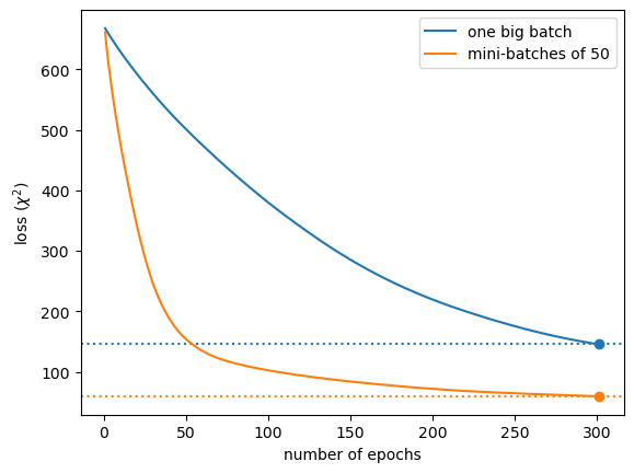
In this and the next code block, we’ll train a 5-hidden layer model, first without mini-batches (all data in one big batch) and then with mini-batches. In both cases, we’ll set the torch.manual_seed to make sure that both optimization processes start in the same state, since random luck can also contribute to the time needed for convergence.
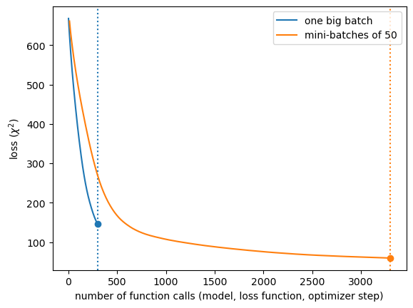
Also, let’s track the value of the loss function and number of function calls (model, loss_function, and optimizer.step()) as a function of epoch.
torch.manual_seed(12345)

NUMBER_OF_EPOCHS = 300

model = nn.Sequential(
    nn.Linear(features.shape[1], 5),         # 13 input features → 5 hidden layers
    nn.ReLU(),                               # activation function
    nn.Linear(5, 1),                         # 5 hidden layers → 1 output prediction
)

loss_function = nn.MSELoss(reduction="sum")  # χ² regression without dividing by N
optimizer = optim.Adam(model.parameters())   # default optimizer

number_of_function_calls = 0
function_calls_vs_epoch = []
loss_vs_epoch = []

for epoch in range(NUMBER_OF_EPOCHS):
    optimizer.zero_grad()

    predictions = model(features)
    loss = loss_function(predictions, targets)

    loss.backward()
    optimizer.step()
    number_of_function_calls += 1

    function_calls_vs_epoch.append(number_of_function_calls)
    loss_vs_epoch.append(loss.item())
Now we’ll do exactly the same thing, but with a mini-batch size of 50.
Calculating the total loss of one epoch takes some care because the output of loss_function is smaller when we give it less data. For this regression problem, nn.MSELoss with reduction="sum" is
so if \(N\) is 1/10th of the size of the dataset, then this \(\chi^2\) will be roughly 1/10ᵗʰ of the total \(\chi^2\).
torch.manual_seed(12345)

NUMBER_OF_EPOCHS = 300
NUMBER_IN_BATCH = 50

model = nn.Sequential(
    nn.Linear(features.shape[1], 5),         # 13 input features → 5 hidden layers
    nn.ReLU(),                               # activation function
    nn.Linear(5, 1),                         # 5 hidden layers → 1 output prediction
)

loss_function = nn.MSELoss(reduction="sum")  # χ² regression without dividing by N
optimizer = optim.Adam(model.parameters())   # default optimizer

number_of_function_calls = 0
function_calls_vs_epoch_batched = []
loss_vs_epoch_batched = []

for epoch in range(NUMBER_OF_EPOCHS):
    total_loss = 0

    for batch_start in range(0, len(features), NUMBER_IN_BATCH):
        batch_stop = batch_start + NUMBER_IN_BATCH

        features_subset = features[batch_start:batch_stop]
        targets_subset = targets[batch_start:batch_stop]

        optimizer.zero_grad()

        predictions = model(features_subset)
        loss = loss_function(predictions, targets_subset)

        loss.backward()
        optimizer.step()
        number_of_function_calls += 1

        total_loss += loss.item()

    function_calls_vs_epoch_batched.append(number_of_function_calls)
    loss_vs_epoch_batched.append(total_loss)
fig, ax = plt.subplots()

ax.plot(range(1, len(loss_vs_epoch) + 1), loss_vs_epoch, label="one big batch")
ax.plot(range(1, len(loss_vs_epoch_batched) + 1), loss_vs_epoch_batched, label=f"mini-batches of {NUMBER_IN_BATCH}")

ax.scatter([len(loss_vs_epoch) + 1], [loss_vs_epoch[-1]], color="tab:blue")
ax.scatter([len(loss_vs_epoch_batched) + 1], [loss_vs_epoch_batched[-1]], color="tab:orange")
ax.axhline(loss_vs_epoch[-1], c="tab:blue", ls=":", zorder=-1)
ax.axhline(loss_vs_epoch_batched[-1], c="tab:orange", ls=":", zorder=-1)

ax.set_xlabel("number of epochs")
ax.set_ylabel("loss ($\chi^2$)")

ax.legend(loc="upper right")

plt.show()

Above, we see that the mini-batched procedure takes about 50 epochs to train as well as 300 epochs with one big batch. (Note: the mini-batch size is 50.)
If you’re trying to minimize the number of times you have to iterate through the data, batching is a big improvement.
fig, ax = plt.subplots()

ax.plot(function_calls_vs_epoch, loss_vs_epoch, label="one big batch")
ax.plot(function_calls_vs_epoch_batched, loss_vs_epoch_batched, label=f"mini-batches of {NUMBER_IN_BATCH}")

ax.scatter([function_calls_vs_epoch[-1]], [loss_vs_epoch[-1]], color="tab:blue")
ax.scatter([function_calls_vs_epoch_batched[-1]], [loss_vs_epoch_batched[-1]], color="tab:orange")
ax.axvline(function_calls_vs_epoch[-1], c="tab:blue", ls=":", zorder=-1)
ax.axvline(function_calls_vs_epoch_batched[-1], c="tab:orange", ls=":", zorder=-1)

ax.set_xlabel("number of function calls (model, loss function, optimizer step)")
ax.set_ylabel("loss ($\chi^2$)")

ax.legend(loc="upper right")

plt.show()

Above, we see that one big batch converges more quickly for the same number of function calls: evaluating the model, the loss function, propagating derivatives, and taking the next step in the optimizer.
If you’re trying to minimize the number of times these functions need to be called, batching is not an improvement.
Optimizing for computational performance#
Ultimately, you want to minimize the amount of time the computer spends training your model, or possibly the total energy use, which is nearly the same thing (ref).
If the whole dataset does not fit in the processor’s working memory, then some kind of batching will be necessary just to compute the model and loss function. Most of the processes involved, such as
reading from disk or network,
decompressing,
reformatting/pre-processing,
copying between memory units, such as RAM → CPU cache or RAM → GPU
are much more expensive than almost any conceivable model. Thus, you’ll generally do better to pass the batches of data that you get from the source into the training step to update the optimization state as much as possible with the data you have, before undertaking the time-consuming step of accumulating the next batch.
Generally, a good mini-batch size for minimizing training time is just small enough for the working memory to fit within your processor’s memory size, such as the GPU global memory. If you’re tuning other hyperparameters, such as learning rate, the numbers of layers and hidden layer sizes, and regularization, re-tune the mini-batch size last, since it depends on all of the rest.
Optimizing for model generalizability#
There’s another reason to train in small batches: it helps to avoid getting stuck in local minima and end up with a model that generalizes well.
In problem domains like stock market prediction, models need to be updated with every new data point: this is called online machine learning. It’s an extreme form of mini-batching in which the NUMBER_IN_BATCH is 1. Each new data point pulls the fitter toward a different minimum, but roughly in the same direction, and this noise prevents the model from memorizing specific features of a constant dataset. Due to the success that online training processes have had over fixed-dataset processes, we’d expect to find some balance between very noisy online training and smooth-but-biased full-dataset training. We’ll discuss techniques to measure overfitting in later sections, but reducing the batch size is one way to reduce overfitting.
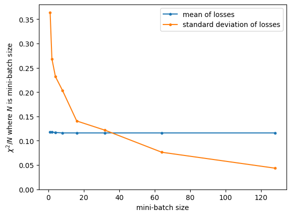
Let’s see the “roughness” of the loss function as a function of batch size for our sample problem. We’ll use the model that has already been optimized above, so we’re near one of its minima.
def losses(batch_size):
    losses = []

    for batch_start in range(0, len(features), batch_size):
        batch_stop = batch_start + batch_size

        features_subset = features[batch_start:batch_stop]
        targets_subset = targets[batch_start:batch_stop]

        predictions = model(features_subset)
        loss = loss_function(predictions, targets_subset)

        losses.append(loss.item() / (batch_stop - batch_start))  # χ²/N

    return losses
fig, ax = plt.subplots()

batch_sizes = [2**x for x in range(int(np.log2(len(features))))]
mean_losses = [np.mean(losses(batch_size)) for batch_size in batch_sizes]
std_losses = [np.std(losses(batch_size)) for batch_size in batch_sizes]

ax.plot(batch_sizes, mean_losses, marker=".", label="mean of losses")
ax.plot(batch_sizes, std_losses, marker=".", label="standard deviation of losses")

ax.set_ylim(0, ax.get_ylim()[1])
ax.set_xlabel("mini-batch size")
ax.set_ylabel("$\chi^2/N$ where $N$ is mini-batch size")

ax.legend(loc="upper right")

plt.show()

As the mini-batch size increases, the calculation of loss becomes more stable. For this dataset and this model, it’s more stable than the (already optimized) value of loss itself when mini-batch sizes are above 40 or 50.
Just keep in mind that the proper way to tune a model for generalizability is to use a validation dataset, which we’ll discuss in an upcoming section.
