Introduction
Overview
Teaching: 10 min
Exercises: 1 minQuestions
What makes research data analyses reproducible?
Is preserving code, data, and containers enough?
Objectives
Understand principles behind computational reproducibility
Understand the concept of serial and parallel computational workflow graphs
Computational reproducibility
A reproducibility quote
An article about computational science in a scientific publication is not the scholarship itself, it is merely advertising of the scholarship. The actual scholarship is the complete software development environment and the complete set of instructions which generated the figures.
– Jonathan B. Buckheit and David L. Donoho, “WaveLab and Reproducible Research”, source
Computational reproducibility has many definitions. Terms such as reproducibility, replicability, and repeatability often have different meanings in different scientific disciplines.
One perspective on computational reproducibility is provided by The Turing Way: source
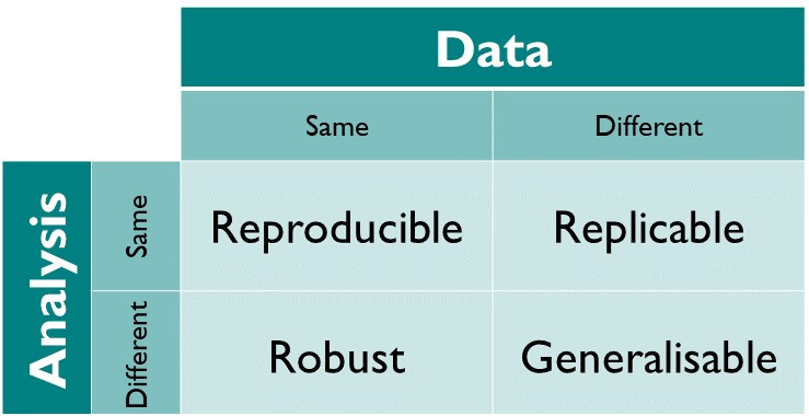
In other words, “same data + same analysis = reproducible results” (perhaps run on a different underlying computing architecture such as from Intel to ARM processors).
The more interesting use case is “reusable analyses”, i.e. testing the same theory on new data, or altering the theory and reinterpreting old data.
Another perspective on computational reproducibility is provided by the PRIMAD model: source
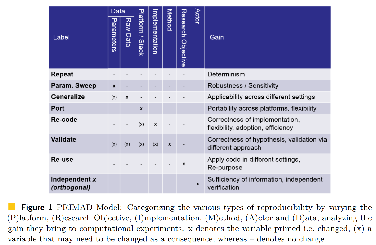
An analysis is reproducible, repeatable, reusable, robust if one can “wiggle” various parameters entering the process. For example, change platform (from Intel to ARM processors); is it portable? Or change the actor performing the analysis (from Alice to Bob); is it independent of the analyst?
In practice, it often is not.
For example, Monya Baker published in Nature 533 (2016) 452–454 the results of surveying 1,500 scientists: source
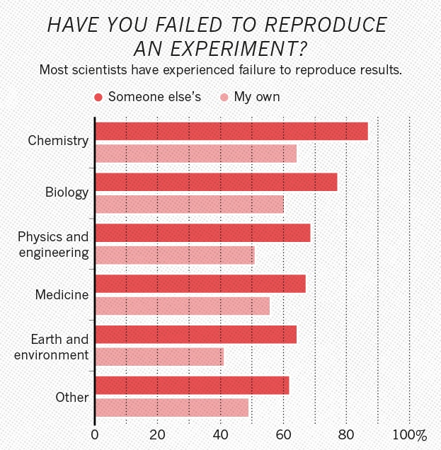
Half of researchers cannot reproduce even their own results. And physics is not doing visibly better than the other scientific disciplines.
Slow uptake of best practices
Many guidelines with “best practices” for computational reproducibility have been published. For example, “Ten Simple Rules for Reproducible Computational Research” by Geir Kjetil Sandve, Anton Nekrutenko, James Taylor, Eivind Hovig (2013) DOI:10.1371/journal.pcbi.1003285:
- For every result, keep track of how it was produced
- Avoid manual data manipulation steps
- Archive the exact versions of all external programs used
- Version control all custom scripts
- Record all intermediate results, when possible in standardized formats
- For analyses that include randomness, note underlying random seeds
- Always store raw data behind plots
- Generate hierarchical analysis output, allowing layers of increasing detail to be inspected
- Connect textual statements to underlying results
- Provide public access to scripts, runs, and results
Yet the uptake of good practices in real life has been slow. There are several reasons, including:
- sociological: publish-or-perish culture in scientific careers; missing incentives to create robust preserved and reusable technology stack;
- technological: easy-to-use tools for “active analyses” that facilitate their future reuse.
The change is being brought about by a combination of top-down approaches (e.g. funding bodies asking for Data Management Plans) and bottom-up approaches (building tools that integrate into daily research workflows).
A reproducibility quote
Your closest collaborator is you six months ago… and your younger self does not reply to emails.
Four questions
Four questions to aid assessing the robustness of analyses:
- Where is your input data? Specify all input data and input parameters that the analysis uses.
- Where is your analysis code? Specify the analysis code and the software frameworks that are being used to analyse the data.
- Which computing environment do you use? Specify the operating system platform that is used to run the analysis.
- What are the computational steps to achieve the results? Specify all the commands and GUI clicks necessary to arrive at the final results.
The input data for statistical analyses, such as CMS MiniAOD, is produced centrally, and its location is well-known.
The analysis code and the containerised computational environments were covered in the previous two days of this workshop:
Exercise
Are containers enough to capture your runtime environment? What else might be necessary in your typical physics analysis scenarios?
Solution
Any external resources, such as condition database calls, must also be thought about. Will the external database that you use still be there and answering queries in the future?
Computational steps
Today’s lesson will focus mostly on the fourth question, i.e. the preservation of running computational steps.
The use of interactive and graphical interfaces is not recommended, since one cannot easily capture and reproduce user clicks.
The use of custom helper scripts (e.g. run.sh shell scripts), or custom orchestration scripts
(e.g. Python glue code) running the analysis is much better.
However, porting glue code to new usage scenarios (for example to scale up to a new computing cluster) may be tedious technical work that would be better spent doing physics instead.
Hence the birth of declarative workflow systems that express the computational steps more abstractly.
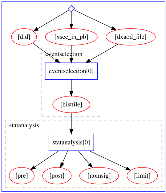
Example of a serial computational workflow graph typical for ATLAS RECAST analyses:
Example of a parallel computational workflow graph typical for Beyond Standard Model searches:
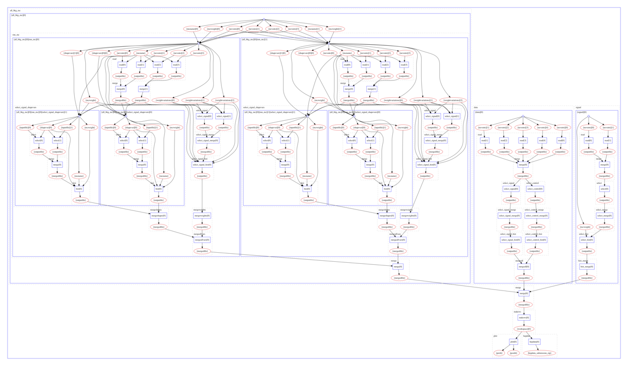
Many different computational data analysis workflow systems exist. Some are preferred to others because of the features they bring that others do not have, so there are fit-for-use and fit-for-purpose considerations. Some are preferred due to cultural differences in research teams or due to individual preferences.
In experimental particle physics, several such workflow systems are being used, for example Snakemake in LHCb or Yadage in ATLAS.
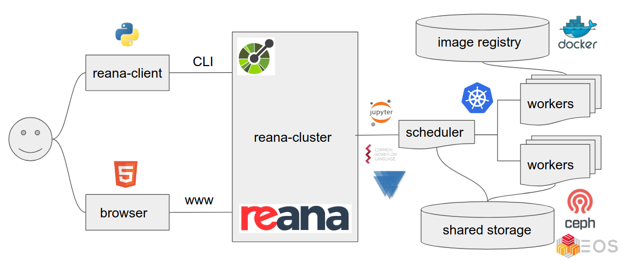
REANA
We shall use the REANA reproducible analysis platform to explore computational workflows in this lesson. REANA supports:
- multiple workflow systems (CWL, Serial, Snakemake, Yadage)
- multiple compute backends (Kubernetes, HTCondor, Slurm)
Analysis preservation ab initio
Preserving analysis code and processes after the publication is often coming too late. The key information and knowledge how to arrive at the results may get lost during the lengthy analysis process.
Hence the idea of making research reproducible from the start, in other words making research “preproducible”, to make the analysis preservation easy.
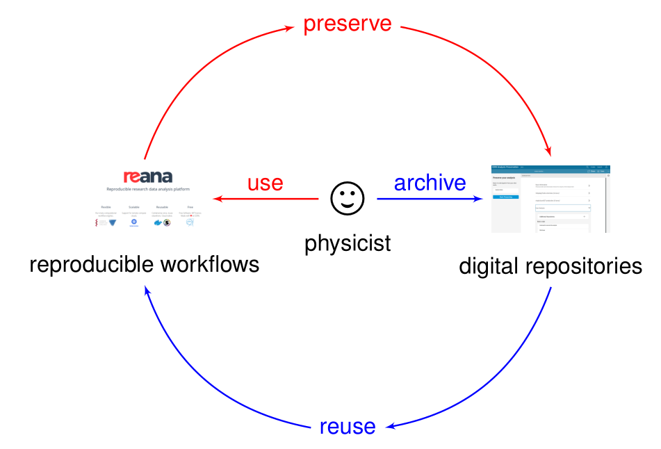
Preserving data first and thinking about reusability later is the “blue pill” way.
Make analysis preproducible ab initio to facilitate its future preservation is the “red pill” way.
Key Points
Workflow is the new data.
Data + Code + Environment + Workflow = Reproducible Analyses
Before reproducibility comes preproducibility
First example
Overview
Teaching: 15 min
Exercises: 5 minQuestions
How to run analyses on REANA cloud?
What are the basic REANA command-line client usage scenarios?
How to monitor my analysis using REANA web interface?
Objectives
Get hands-on experience with REANA command-line client
Overview
In this lesson we shall run our first simple REANA example. We shall see:
- structure of the example analysis and associated
reana.yamlfile - how to install the REANA command-line client
- how to connect REANA client to remote REANA cluster
- how to run analysis on remote REANA cluster
Checklist
Have you installed
reana-clientand/or have you logged into LXPLUS as described in Setup?
First REANA example
We shall get acquainted with REANA by means of running a sample analysis example:
Let’s start by cloning it:
git clone https://github.com/reanahub/reana-demo-root6-roofit
cd reana-demo-root6-roofit
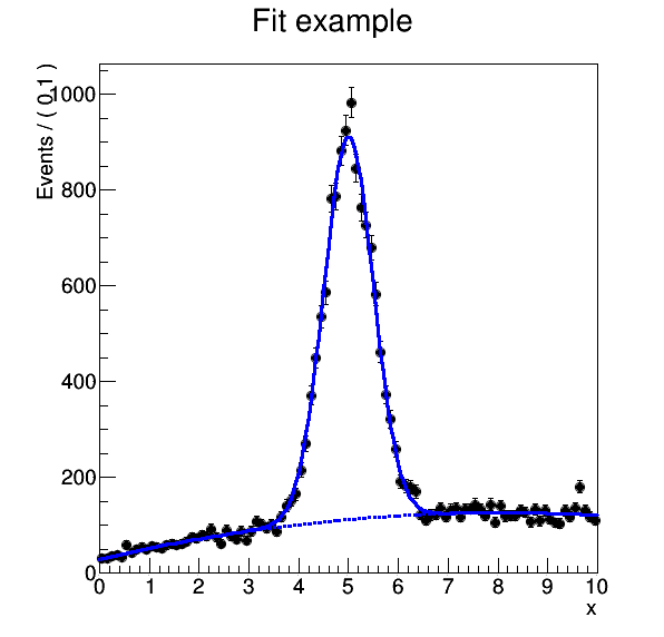
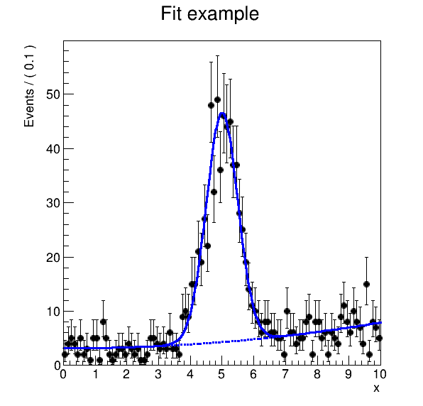
What does the example do? The example emulates a typical particle physics analysis where the signal and background data is processed and fitted against a model. The example uses the RooFit package of the ROOT framework.
Four questions:
- Where is your input data? There is no input data. We shall simulate them.
- Where is your analysis code? Two files:
gendata.Cmacro generates signal and background data;fitdata.Cmacro makes a fit for the signal and the background data. - Which computing environment do you use? ROOT 6.18.04 with RooFit.
- What are the computational steps to achieve the results? Simple sequential steps: first run gendata, then run fitdata.
Workflow definition:
           START
            |
            |
            V
+-------------------------+
| (1) generate data       |
|                         |
|    $ root gendata.C ... |
+-------------------------+
            |
            | data.root
            V
+-------------------------+
| (2) fit data            |
|                         |
|    $ root fitdata.C ... |
+-------------------------+
            |
            | plot.png
            V
           STOP
The four questions expressed in reana.yaml fully define our analysis:
inputs:
  files:
    - code/gendata.C
    - code/fitdata.C
  parameters:
    events: 20000
    data: results/data.root
    plot: results/plot.png
workflow:
  type: serial
  specification:
    steps:
      - name: gendata
        environment: 'docker.io/reanahub/reana-env-root6:6.18.04'
        commands:
        - mkdir -p results && root -b -q 'code/gendata.C(${events},"${data}")'
      - name: fitdata
        environment: 'docker.io/reanahub/reana-env-root6:6.18.04'
        commands:
        - root -b -q 'code/fitdata.C("${data}","${plot}")'
outputs:
  files:
    - results/plot.png
Note the basic structure of reana.yaml answering the Four Questions. (Where is input data? Where
is analysis code? What compute environment to use? What are the computational steps to arrive at
results?)
Exercise
Familiarise yourself with the RooFit demo example by studying the README file and looking at the
gendata.Candfitdata.Csource code.
Solution
firefox https://github.com/reanahub/reana-demo-root6-roofit
First steps with the REANA command-line client
First we need to make sure we can use REANA command-line client. See the setup instructions if you haven’t already installed it.
The client will offer several commands which we shall go through in this tutorial:
reana-client --help
Usage: reana-client [OPTIONS] COMMAND [ARGS]...

  REANA client for interacting with REANA server.

Options:
  -l, --loglevel [DEBUG|INFO|WARNING]
                                  Sets log level
  --help                          Show this message and exit.

Quota commands:
  quota-show  Show user quota.

Configuration commands:
  info     List cluster general information.
  ping     Check connection to REANA server.
  version  Show version.

Workflow management commands:
  create  Create a new workflow.
  delete  Delete a workflow.
  diff    Show diff between two workflows.
  list    List all workflows and sessions.

Workflow execution commands:
  logs      Get workflow logs.
  restart   Restart previously run workflow.
  run       Shortcut to create, upload, start a new workflow.
  start     Start previously created workflow.
  status    Get status of a workflow.
  stop      Stop a running workflow.
  validate  Validate workflow specification file.

Workspace interactive commands:
  close  Close an interactive session.
  open   Open an interactive session inside the workspace.

Workspace file management commands:
  download  Download workspace files.
  du        Get workspace disk usage.
  ls        List workspace files.
  mv        Move files within workspace.
  prune     Prune workspace files.
  rm        Delete files from workspace.
  upload    Upload files and directories to workspace.

Workspace file retention commands:
  retention-rules-list  List the retention rules for a workflow.

Secret management commands:
  secrets-add     Add secrets from literal string or from file.
  secrets-delete  Delete user secrets by name.
  secrets-list    List user secrets.
You can use --help option to learn more about any command, for example validate:
reana-client validate --help
Usage: reana-client validate [OPTIONS]

  Validate workflow specification file.

  The ``validate`` command allows to check syntax and validate the reana.yaml
  workflow specification file.

  Examples:

       $ reana-client validate -f reana.yaml

Options:
  -f, --file PATH          REANA specification file describing the workflow to
                           execute. [default=reana.yaml]
  --environments           If set, check all runtime environments specified in
                           REANA specification file. [default=False]
  --pull                   If set, try to pull remote environment image from
                           registry to perform validation locally. Requires
                           ``--environments`` flag. [default=False]
  --server-capabilities    If set, check the server capabilities such as
                           workspace validation. [default=False]
  -t, --access-token TEXT  Access token of the current user.
  --help                   Show this message and exit.
Exercise
Validate our
reana.yamlfile to discover any errors. Usevalidatecommand to do so.
Solution
reana-client validate==> Verifying REANA specification file... reana.yaml -> SUCCESS: Valid REANA specification file. ==> Verifying REANA specification parameters... -> SUCCESS: REANA specification parameters appear valid. ==> Verifying workflow parameters and commands... -> SUCCESS: Workflow parameters and commands appear valid. ==> Verifying dangerous workflow operations... -> SUCCESS: Workflow operations appear valid.
Connect REANA client to remote REANA cluster
The REANA client will interact with a remote REANA cluster. It knows to which REANA cluster it connects by means of the following environment variable:
export REANA_SERVER_URL=https://reana.cern.ch
In order to authenticate to REANA, you need to generate a token.
Exercise: Obtain a token.
In order to obtain your token, please go to https://reana.cern.ch and ask for it.
In your terminal, paste the line with your new access token as seen below.
export REANA_ACCESS_TOKEN=xxxxxx
It may be a good idea to create a reana-setup-environment.sh file to store these two export
commands. That way you all you need to do to setup your environment is source
reana-setup-environment.sh. An alternative to this is opening up your .bashrc file and pasting
the above two export commands there.
The REANA client connection to remote REANA cluster can be verified via ping command:
reana-client ping
REANA server: https://reana.cern.ch
REANA server version: 0.9.1
REANA client version: 0.9.1
Authenticated as: John Doe <john.doe@example.org>
Status: Connected
Run example on REANA cluster
Now that we have defined and validated our reana.yaml, and connected to the REANA production
cluster, we can run the example easily via:
reana-client run -w roofit
==> Creating a workflow...
==> Verifying REANA specification file... reana.yaml
  -> SUCCESS: Valid REANA specification file.
==> Verifying REANA specification parameters...
  -> SUCCESS: REANA specification parameters appear valid.
==> Verifying workflow parameters and commands...
  -> SUCCESS: Workflow parameters and commands appear valid.
==> Verifying dangerous workflow operations...
  -> SUCCESS: Workflow operations appear valid.
==> Verifying compute backends in REANA specification file...
-> SUCCESS: Workflow compute backends appear to be valid.
roofit.1
==> SUCCESS: File /reana.yaml was successfully uploaded.
==> Uploading files...
==> Detected .gitignore file. Some files might get ignored.
==> SUCCESS: File /code/gendata.C was successfully uploaded.
==> SUCCESS: File /code/fitdata.C was successfully uploaded.
==> Starting workflow...
==> SUCCESS: roofit.1 is pending
Here, we use run command that will create a new workflow named roofit, upload its inputs as
specified in the workflow specification and finally start the workflow.
While the workflow is running, we can enquire about its status:
reana-client status -w roofit
NAME     RUN_NUMBER   CREATED               STARTED               STATUS    PROGRESS
roofit   1            2020-02-17T16:01:45   2020-02-17T16:01:48   running   1/2
After a minute or so, the workflow should finish:
reana-client status -w roofit
NAME     RUN_NUMBER   CREATED               STARTED               ENDED                 STATUS     PROGRESS
roofit   1            2020-02-17T16:01:45   2020-02-17T16:01:48   2020-02-17T16:02:44   finished   2/2
We can list the output files in the remote workspace:
reana-client ls -w roofit
NAME                SIZE     LAST-MODIFIED
reana.yaml          687      2020-02-17T16:01:46
code/gendata.C      1937     2020-02-17T16:01:46
code/fitdata.C      1648     2020-02-17T16:01:47
results/plot.png    15450    2020-02-17T16:02:44
results/data.root   154457   2020-02-17T16:02:17
We can also inspect the logs:
reana-client logs -w roofit | less
# (Hit q to quit 'less')
==> Workflow engine logs
2020-02-17 16:02:10,859 | root | MainThread | INFO | Publishing step:0, cmd: mkdir -p results && root -b -q 'code/gendata.C(20000,"results/data.root")', total steps 2 to MQ
2020-02-17 16:02:23,002 | root | MainThread | INFO | Publishing step:1, cmd: root -b -q 'code/fitdata.C("results/data.root","results/plot.png")', total steps 2 to MQ
2020-02-17 16:02:50,093 | root | MainThread | INFO | Workflow 424bc949-b809-4782-ba96-bc8cfa3e1a89 finished. Files available at /var/reana/users/b57e902f-fd11-4681-8a94-4318ae05d2ca/workflows/424bc949-b809-4782-ba96-bc8cfa3e1a89.

==> Job logs
==> Step: gendata
==> Workflow ID: 424bc949-b809-4782-ba96-bc8cfa3e1a89
==> Compute backend: Kubernetes
==> Job ID: 53c97429-25e9-4b74-94f7-c665d93fdbc2
==> Docker image: reanahub/reana-env-root6:6.18.04
==> Command: mkdir -p results && root -b -q 'code/gendata.C(20000,"results/data.root")'
==> Status: finished
==> Logs:
...
We can download the resulting plot:
reana-client download results/plot.png -w roofit
==> SUCCESS: File results/plot.png downloaded to reana-demo-root6-roofit.
And display it:
firefox results/plot.png
Exercise
Run the example workflow on REANA cluster. Practice
status,ls,logs,downloadcommands. For example, can you get the logs of the gendata step only?
Solution
reana-client logs -w roofit --filter step=gendata
Key Points
Use
reana-clientrich command-line client to run containerised workflows from your laptop on remote compute cloudsBefore running analysis remotely, check locally its correctness via
validatecommandAs always, when it doubt, use the
--helpcommand-line argument
Developing serial workflows
Overview
Teaching: 20 min
Exercises: 10 minQuestions
How to write serial workflows?
What is declarative programming?
How to develop workflows progressively?
Can I temporarily override workflow parameters?
Do I always have to build new Docker image when my code changes?
Objectives
Understand pros/cons between imperative and declarative programming styles
Get familiar with serial workflow development practices
Understand run numbers of your analysis
See how you can run only parts of the workflow
See how you can repeat workflow to fix a failed step
Overview
We have seen how to use REANA client to run containerised analyses on the REANA cloud.
In this lesson we see more use cases suitable for developing serial workflows.
Imperative vs declarative programming
Imperative programming feels natural: use a library and just write code. Example: C.
for (int i = 0; i < sizeof(people) / sizeof(struct people); i++) {
  if (people[i].age < 20) {
    printf("%s\n", people[i].name)
  }
}
However, it also has its drawbacks. If you write scientific workflows imperatively and you need to port the code to run on different compute architectures, or to scale up, it may be necessary to do considerable code refactoring. This is not writing science code, but rather writing orchestration for the said science code onto different deployment scenarios.
Enter declarative programming that “expresses the logic of a computation without describing its control flow”. Example: SQL.
SELECT name FROM people WHERE age<20
The idea of a declarative approach to scientific workflows is to express research as a series of data analysis steps and let an independent “orchestration tool” or a “workflow system” handle the task of running things properly on various deployment architectures.
This achieves better separation of concerns between physics code knowledge and computing orchestration glue code knowledge. However, the development may be felt less immediate. There are pros and cons. There is no silver bullet.
Imperative or declarative?
Imperative programming is about how you want to achieve something. Declarative programming is about what you want to achieve.
Developing workflows progressively
Developing workflows declaratively may feel less natural. How do we do that?
Start with earlier steps, then run, debug, and iterate until satisfied.
Only then continue with later steps.
How do we run only the first step of our example workflow? Use the TARGET step option:
reana-client run -w roofit -o TARGET=gendata
==> Creating a workflow...
==> Verifying REANA specification file... reana.yaml
  -> SUCCESS: Valid REANA specification file.
==> Verifying REANA specification parameters...
  -> SUCCESS: REANA specification parameters appear valid.
==> Verifying workflow parameters and commands...
  -> SUCCESS: Workflow parameters and commands appear valid.
==> Verifying dangerous workflow operations...
  -> SUCCESS: Workflow operations appear valid.
==> Verifying compute backends in REANA specification file...
  -> SUCCESS: Workflow compute backends appear to be valid.
roofit.2
==> SUCCESS: File /reana.yaml was successfully uploaded.
==> Uploading files...
==> Detected .gitignore file. Some files might get ignored.
==> SUCCESS: File /code/fitdata.C was successfully uploaded.
==> SUCCESS: File /code/gendata.C was successfully uploaded.
==> Starting workflow...
==> SUCCESS: roofit.2 has been queued
After a minute, let us check the status:
reana-client status -w roofit
NAME     RUN_NUMBER   CREATED               STARTED               ENDED                 STATUS     PROGRESS
roofit   2            2020-02-17T16:07:29   2020-02-17T16:07:33   2020-02-17T16:08:48   finished   1/2
and the workspace content:
reana-client ls -w roofit
NAME                SIZE     LAST-MODIFIED
reana.yaml          687      2020-02-11T16:07:30
code/gendata.C      1937     2020-02-17T16:07:30
code/fitdata.C      1648     2020-02-17T16:07:31
results/data.root   154458   2020-02-17T16:08:43
As we can see, the workflow ran only the first command and the data.root file was successfully
generated. The final fitting step was not run and the final plot was not produced.
Workflow runs
We have run the analysis example anew. Similar to Continuous Integration systems, the REANA platform
runs each workflow in an independent workspace. To distinguish between various workflow runs of the
same analysis, the REANA platform keeps an incremental “run number”. You can obtain the list of all
your workflows by using the list command:
reana-client list
NAME     RUN_NUMBER   CREATED               STARTED               ENDED                 STATUS
roofit   2            2020-02-17T16:07:29   2020-02-17T16:07:33   2020-02-17T16:08:48   finished
roofit   1            2020-02-17T16:01:45   2020-02-17T16:01:48   2020-02-17T16:02:50   finished
You can use myanalysis.myrunnumber to refer to a given run number of an analysis:
reana-client ls -w roofit.1
reana-client ls -w roofit.2
To quickly know the differences between various workflow runs, you can use the diff command:
reana-client diff roofit.1 roofit.2 --brief
==> No differences in REANA specifications.

==> Differences in workflow workspace
Files roofit.1/results/data.root and roofit.2/results/data.root differ
Only in roofit.1/results: plot.png
Workflow parameters
Another useful technique when developing a workflow is to use smaller data samples until the workflow is debugged. For example, instead of generating 20000 events, we can generate only 1000. While you could achieve this by simply modifying the workflow definition, REANA offers an option to run parametrised workflows, meaning that you can pass the wanted value on the command line:
reana-client run -w roofit -p events=1000
==> Creating a workflow...
==> Verifying REANA specification file... /home/tibor/private/project/reana/src/reana-demo-root6-roofit/reana.yaml
  -> SUCCESS: Valid REANA specification file.
==> Verifying REANA specification parameters...
  -> SUCCESS: REANA specification parameters appear valid.
==> Verifying workflow parameters and commands...
  -> SUCCESS: Workflow parameters and commands appear valid.
==> Verifying dangerous workflow operations...
  -> SUCCESS: Workflow operations appear valid.
==> Verifying compute backends in REANA specification file...
  -> SUCCESS: Workflow compute backends appear to be valid.
roofit.3
==> SUCCESS: File /reana.yaml was successfully uploaded.
==> Uploading files...
==> Detected .gitignore file. Some files might get ignored.
==> SUCCESS: File /code/gendata.C was successfully uploaded.
==> SUCCESS: File /code/fitdata.C was successfully uploaded.
==> Starting workflow...
==> SUCCESS: roofit.3 has been queued
The generated ROOT file is much smaller:
reana-client ls -w roofit.1 | grep data.root
results/data.root 154457 2020-02-17T16:02:17
reana-client ls -w roofit.3 | grep data.root
results/data.root 19216 2020-02-17T16:18:45
and the plot much coarser:
reana-client download results/plot.png -w roofit.3
Developing further steps
Now that we are happy with the beginning of the workflow, how do we continue to develop the rest? Running a new workflow every time could be very time consuming; running skimming may require many more minutes than running statistical analysis.
In these situations, you can take advantage of the restart functionality. The REANA platform
allows to restart a part of the workflow on the given workspace starting from the workflow step
specified by the FROM option:
reana-client restart -w roofit.3 -o FROM=fitdata
==> SUCCESS: roofit.3.1 is pending
Note that the run number got an extra digit, meaning the number of restarts of the given workflow.
The full semantics of REANA run numbers is myanalysis.myrunnumber.myrestartnumber.
Let us enquire about the status of the restarted workflow:
reana-client status -w roofit.3.1
NAME     RUN_NUMBER   CREATED               STARTED               ENDED                 STATUS     PROGRESS
roofit   3.1          2020-02-17T16:26:09   2020-02-17T16:26:10   2020-02-17T16:27:24   finished   1/2
Looking at the number of steps of the 3.1 rerun, and looking at modification timestamps of the workspace files:
reana-client ls -w roofit.3.1
NAME                SIZE    LAST-MODIFIED
reana.yaml          687     2020-02-17T16:17:00
code/gendata.C      1937    2020-02-17T16:17:00
code/fitdata.C      1648    2020-02-17T16:17:01
results/plot.png    16754   2020-02-17T16:27:20
results/data.root   19216   2020-02-17T16:18:45
We can see that only the last step of the workflow was rerun, as wanted.
This technique is useful to debug later stages of the workflow without having to rerun the lengthy former stages of the workflow.
Exercise
Consider we would like to produce the final plot of the roofit example and change the title from “Fit example” to “RooFit example”. How do you do this in the most efficient way?
Solution
Amend
fitdata.C, upload changed file to the workspace, and rerun the past successful workflow starting from the fitdata step:reana-client list vim code/fitdata.C # edit title printing statement reana-client upload ./code/fitdata.C -w roofit.3 reana-client restart -w roofit.3 -o FROM=fitdata reana-client list reana-client status -w roofit.3.2 reana-client download -w roofit.3.2
Compile-time vs runtime code changes
Sometimes you have to build a new container image when code changes (e.g. C++ compilation); sometimes you don’t (e.g. Python code, ROOT macros). Use the latter for more productivity when developing workflows.
Key Points
Develop workflows progressively; add steps as needed
When developing a workflow, stay on the same workspace
When developing a bytecode-interpreted code, stay on the same container
Use smaller test data before scaling out
Use workflows as Continuous Integration; make atomic commits that always work
HiggsToTauTau analysis: serial
Overview
Teaching: 5 min
Exercises: 20 minQuestions
Challenge: write the HiggsToTauTau analysis workflow and run it on REANA
Objectives
Develop a full HiggsToTauTau analysis workflow using a simple serial language
Get acquainted with writing moderately complex REANA examples
Overview
In the previous two episodes we have practised writing and running workflows on REANA using a simple RooFit analysis example.
In this episode we shall go back to the HiggsToTauTau analysis example that you used throughout the workshop and we shall write a serial workflow to run this analysis on the REANA platform.
Recap
In the past two days of this workshop you have followed two lessons:
The lessons were using a HiggsToTauTau example analysis described in detail here:
You have containerised this analysis by means of two GitLab repositories:
gitlab.cern.ch/johndoe/awesome-analysis-eventselectioncontaining the skimming and histogramming;gitlab.cern.ch/johndoe/awesome-analysis-statisticscontaining the statistical modelling and fitting.
You have used the GitLab CI/CD to build the Docker images for these repositories and published them as:
gitlab-registry.cern.ch/johndoe/awesome-analysis-eventselection:master-sha1agitlab-registry.cern.ch/johndoe/awesome-analysis-statistics:master-sha1b
You have run the containerised HiggsToTauTau analysis “manually” by using docker commands for
various analysis steps such as:
bash skim.sh ...bash histograms.sh ...bash plot.sh ...bash fit.sh ...
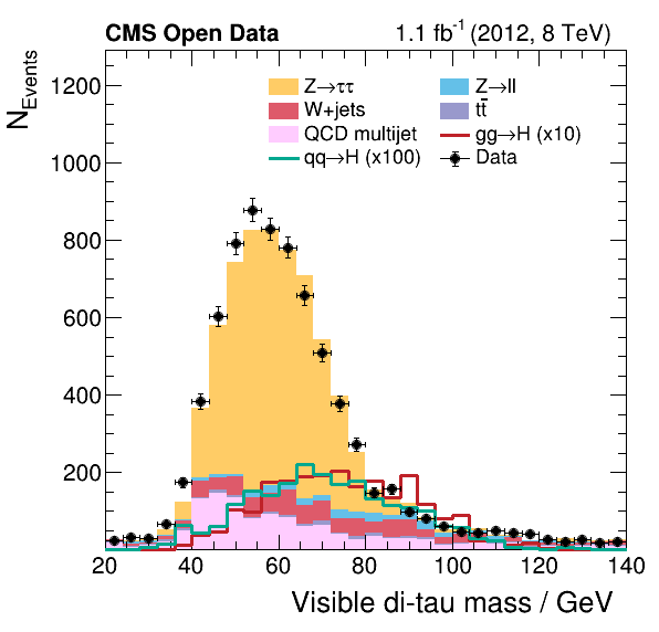
And you have produced the plots and the fit:

If you haven’t fully followed the previous lessons on Docker and GitLab CI/CD…
Note that if you haven’t fully followed the previous lessons on Docker and GitLab CI/CD and so you haven’t produced your own container images
gitlab.cern.ch/johndoe/awesome-analysis-eventselectionandgitlab.cern.ch/johndoe/awesome-analysis-statistics, you can follow the rest of the episodes in this lesson using the following example imagesgitlab-registry.cern.ch/awesome-workshop/awesome-analysis-eventselection-stage3:masterandgitlab-registry.cern.ch/awesome-workshop/awesome-analysis-statistics-stage3:master. It is these images that we shall use in the solutions to the exercises below.
Objective
Let us write a serial computational workflow automating the previously-run manual steps and run the HiggsToTauTau example on REANA.
Note: Computing efficiency
Note that the serial workflow will not be necessarily efficient here, since it will run sequentially over various dataset files and not process them in parallel. Do not pay attention to this inefficiency here yet. We shall speed up the serial example via parallel processing in the forthcoming HiggsToTauTau analysis: parallel episode coming after the coffee break.
Note: Container directories and workspace directories
The awesome-analysis-eventselection and awesome-analysis-statistics repositories assume that you
run code from certain absolute directories such as /analysis/skim. Recall that when REANA starts
a new workflow run, it creates a certain unique “workspace directory” and uses it as the default
directory for all the analysis steps throughout the workflow, allowing to share read/write files
amongst the steps.
It is a good practice to consider the absolute directories in your container images such as
/analysis/skim as read-only and rather use the dynamic workflow’s workspace for any writeable
needs. In this way, we don’t risk to write over any code or configuration files provided by the
container. This is good both for reproducibility and security purposes.
Moreover, writing into the running container would increase its size unnecessarily. Writing to the dynamic workspace that is mounted inside the container keeps the container size small.
Note: REANA_WORKSPACE environment variable
REANA platform uses a convenient set of environment variables that you can use in your scripts. One
of them is REANA_WORKSPACE which points to the workflow’s workspace which is uniquely allocated
for each run. You can use the $$REANA_WORKSPACE environment variable in your reana.yaml recipe
to share the output of skimming, histogramming, plotting and fitting steps. (Note the use of two
leading dollar signs to escape the workflow parameter expansion that you have used in the previous
episodes.)
OK, challenge time!
With the above hints in mind, please try to write the workflow either individually or in pairs.
Exercise
Write
reana.yamlrepresenting HiggsToTauTau analysis and run it on the REANA cloud.
Solution
inputs:
  parameters:
    eosdir: root://eospublic.cern.ch//eos/root-eos/HiggsTauTauReduced
workflow:
  type: serial
  specification:
    steps:
      - name: skimming
        environment: gitlab-registry.cern.ch/awesome-workshop/awesome-analysis-eventselection-stage3:master
        commands:
          - mkdir $$REANA_WORKSPACE/skimming && cd /analysis/skim && bash ./skim.sh ${eosdir} $$REANA_WORKSPACE/skimming
      - name: histogramming
        environment: gitlab-registry.cern.ch/awesome-workshop/awesome-analysis-eventselection-stage3:master
        commands:
          - mkdir $$REANA_WORKSPACE/histogramming && cd /analysis/skim && bash ./histograms_with_custom_output_location.sh $$REANA_WORKSPACE/skimming $$REANA_WORKSPACE/histogramming
      - name: plotting
        environment: gitlab-registry.cern.ch/awesome-workshop/awesome-analysis-eventselection-stage3:master
        commands:
          - mkdir $$REANA_WORKSPACE/plotting && cd /analysis/skim && bash ./plot.sh $$REANA_WORKSPACE/histogramming/histograms.root $$REANA_WORKSPACE/plotting 0.1
      - name: fitting
        environment: gitlab-registry.cern.ch/awesome-workshop/awesome-analysis-statistics-stage3:master
        commands:
          - mkdir $$REANA_WORKSPACE/fitting && cd /fit && bash ./fit.sh $$REANA_WORKSPACE/histogramming/histograms.root $$REANA_WORKSPACE/fitting
outputs:
  files:
    - fitting/fit.png
Key Points
Writing serial workflows is like chaining shell script commands
Coffee break
Overview
Teaching: 15 min
Exercises: 0 minQuestions
Coffee break
Objectives
Refresh your mind
Discuss your experience

Key Points
Refresh your mind
Discuss your experience
Developing parallel workflows
Overview
Teaching: 15 min
Exercises: 10 minQuestions
How to scale up and run thousands of jobs?
What is a DAG?
What is a Scatter-Gather paradigm?
How to run Yadage workflows on REANA?
Objectives
Learn about Directed Acyclic Graphs (DAG)
Understand Yadage workflow language
Practice running and inspecting parallel workflows
Overview
We now know how to develop reproducible analyses on small scale using serial workflows.
In this lesson we shall learn how to scale up for real-life work which usually requires using parallel workflows.
Computational workflows as Directed Acyclic Graphs (DAG)
Computational workflows can be expressed as a set of computational steps where some steps depend on other steps before they can begin their computations. In other words, the computational steps constitute a Directed Acyclic Graph (DAG) where each graph vertex represents a unit of computation with its inputs and outputs, and the graph edges describe the interconnections between computational steps. For example:
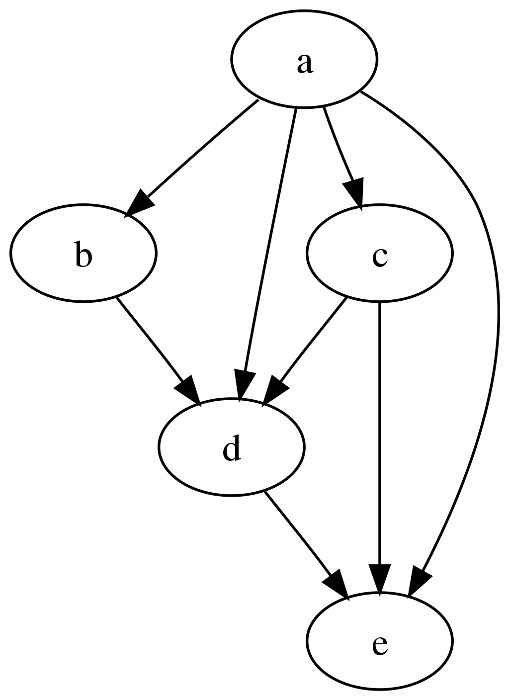
The graph is “directed” and “acyclic” because it can be topologically ordered so that later steps depend on earlier steps without cyclic dependencies, with progress flowing steadily from earlier steps to later steps.
The REANA platform supports several DAG workflow specification languages:
- Common Workflow Language (CWL) originated in life sciences;
- Snakemake originated in bioinformatics;
- Yadage originated in particle physics.
Workflow specification languages
The examples in this lesson use Snakemake (used e.g. in LHCb) and Yadage (used e.g. in ATLAS). Select a tab below to see the RooFit example expressed in each language.
Yadage enables describing even very complex computational workflows. Here is the Yadage specification for the RooFit example used in the previous episodes:
stages:
  - name: gendata
    dependencies: [init]
    scheduler:
      scheduler_type: 'singlestep-stage'
      parameters:
        events: {step: init, output: events}
        gendata: {step: init, output: gendata}
        outfilename: '{workdir}/data.root'
      step:
        process:
          process_type: 'interpolated-script-cmd'
          script: root -b -q '{gendata}({events},"{outfilename}")'
        publisher:
          publisher_type: 'frompar-pub'
          outputmap:
            data: outfilename
        environment:
          environment_type: 'docker-encapsulated'
          image: 'docker.io/reanahub/reana-env-root6'
          imagetag: '6.18.04'
  - name: fitdata
    dependencies: [gendata]
    scheduler:
      scheduler_type: 'singlestep-stage'
      parameters:
        fitdata: {step: init, output: fitdata}
        data: {step: gendata, output: data}
        outfile: '{workdir}/plot.png'
      step:
        process:
          process_type: 'interpolated-script-cmd'
          script: root -b -q '{fitdata}("{data}","{outfile}")'
        publisher:
          publisher_type: 'frompar-pub'
          outputmap:
            plot: outfile
        environment:
          environment_type: 'docker-encapsulated'
          image: 'docker.io/reanahub/reana-env-root6'
          imagetag: '6.18.04'
We can see that the workflow consists of two stages, the gendata stage that does not depend on
anything (this is denoted by [init] dependency which means the stage can run right after the
workflow initialisation already), and the fitdata stage that depends on the completion of the
gendata stage (this is denoted by [gendata]).
Note that each stage consists of a single workflow step (singlestep-stage) which represents the
basic unit of computation of the workflow. (We shall see below an example of a multi-step stages
which express the same basic unit of computations scattered over inputs.)
The step consists of the description of the process to run, the containerised environment in which to run the process, as well as the mapping of its outputs to the stage.
This is how the Yadage workflow engine understands which stages can be run in which order, what commands to run in each stage, and how to pass inputs and outputs between steps.
Snakemake uses “rules” where each rule defines its inputs and outputs and the command to run to produce them. The Snakemake workflow engine then computes the dependencies between rules based on how the outputs from some rules are used as inputs to other rules.
rule all:
    input:
        "results/data.root",
        "results/plot.png"

rule gendata:
    output:
        "results/data.root"
    params:
        events=20000
    container:
        "docker://docker.io/reanahub/reana-env-root6:6.18.04"
    shell:
        "mkdir -p results && root -b -q 'code/gendata.C({params.events},\"{output}\")'"

rule fitdata:
    input:
        data="results/data.root"
    output:
        "results/plot.png"
    container:
        "docker://docker.io/reanahub/reana-env-root6:6.18.04"
    shell:
        "root -b -q 'code/fitdata.C(\"{input.data}\",\"{output}\")'"
We see that the final plot is produced by the “fitdata” rule, which needs “data.root” file to be
present, and it is the “gendata” rule that produces it. Hence Snakemake knows that it has to run
the “gendata” rule first, and the computation of “fitdata” is deferred until “gendata” successfully
completes. This process is very similar to how Makefile are being used in Unix software packages.
Running on REANA
We have to instruct REANA which workflow engine to use by editing reana.yaml. Select a tab
below to see the configuration for each engine.
inputs:
  files:
    - code/gendata.C
    - code/fitdata.C
    - workflow.yaml
  parameters:
    events: 20000
    gendata: code/gendata.C
    fitdata: code/fitdata.C
workflow:
  type: yadage
  file: workflow.yaml
outputs:
  files:
    - results/plot.png
Here, workflow.yaml is a new file with the same content as specified above.
Exercise
Run RooFit example using Yadage workflow engine on the REANA cloud. Upload code, run workflow, inspect status, check logs, download final plot.
Solution
Nothing changes in the usual user interaction with the REANA platform:
reana-client create -w my-workflow -f ./reana.yaml
reana-client upload ./code -w my-workflow
reana-client start -w my-workflow
reana-client status -w my-workflow
reana-client logs -w my-workflow
reana-client ls -w my-workflow
reana-client download results/plot.png -w my-workflow
inputs:
  files:
    - code/gendata.C
    - code/fitdata.C
    - Snakefile
workflow:
  type: snakemake
  file: Snakefile
outputs:
  files:
    - results/plot.png
Here, Snakefile is a new file with the same content as specified above.
Exercise
Run RooFit example using Snakemake workflow engine on the REANA cloud. Upload code, run workflow, inspect status, check logs, download final plot.
Solution
Nothing changes in the usual user interaction with the REANA platform:
reana-client create -w my-workflow -f ./reana.yaml
reana-client upload ./code -w my-workflow
reana-client start -w my-workflow
reana-client status -w my-workflow
reana-client logs -w my-workflow
reana-client ls -w my-workflow
reana-client download results/plot.png -w my-workflow
Physics code vs orchestration code
Note that it wasn’t necessary to change anything in our research code: we simply modified the workflow definition and could run the RooFit code “as is” using a different workflow engine. This is a simple demonstration of the separation of concerns between “physics code” and “orchestration code”.
Parallelism via step dependencies
We have seen how the sequential workflows were expressed in the Snakemake/Yadage syntax using stage dependencies. Note that if the stage dependency graph would have permitted, the workflow steps not depending on each other, or on the results of previous computations, would have been executed in parallel by the workflow engine out of the box. The physicist only needs to specify which steps depend on which others, and the workflow engine takes care of efficiently starting and scheduling tasks as necessary.
HiggsToTauTau analysis: simple version
Let us demonstrate how to write a workflow for the HiggsToTauTau example analysis using simple step dependencies. Select a tab below to see the workflow expressed in each language.
The workflow stages look like:
stages:
- name: skim
  dependencies: [init]
  scheduler:
    scheduler_type: singlestep-stage
    parameters:
      input_dir: {step: init, output: input_dir}
      output_dir: '{workdir}/output'
    step: {$ref: 'steps.yaml#/skim'}

- name: histogram
  dependencies: [skim]
  scheduler:
    scheduler_type: singlestep-stage
    parameters:
      input_dir: {step: skim, output: skimmed_dir}
      output_dir: '{workdir}/output'
    step: {$ref: 'steps.yaml#/histogram'}

- name: fit
  dependencies: [histogram]
  scheduler:
    scheduler_type: singlestep-stage
    parameters:
      histogram_file: {step: histogram, output: histogram_file}
      output_dir: '{workdir}/output'
    step: {$ref: 'steps.yaml#/fit'}

- name: plot
  dependencies: [histogram]
  scheduler:
    scheduler_type: singlestep-stage
    parameters:
      histogram_file: {step: histogram, output: histogram_file}
      output_dir: '{workdir}/output'
    step: {$ref: 'steps.yaml#/plot'}
where steps are expressed as:
skim:
  process:
    process_type: 'interpolated-script-cmd'
    script: |
      mkdir {output_dir}
      bash skim.sh {input_dir} {output_dir}
  environment:
    environment_type: 'docker-encapsulated'
    image: gitlab-registry.cern.ch/awesome-workshop/awesome-analysis-eventselection-stage3
    imagetag: master
  publisher:
    publisher_type: interpolated-pub
    publish:
      skimmed_dir: '{output_dir}'

histogram:
  process:
    process_type: 'interpolated-script-cmd'
    script: |
      mkdir {output_dir}
      bash histograms_with_custom_output_location.sh {input_dir} {output_dir}
  environment:
    environment_type: 'docker-encapsulated'
    image: gitlab-registry.cern.ch/awesome-workshop/awesome-analysis-eventselection-stage3
    imagetag: master
  publisher:
    publisher_type: interpolated-pub
    publish:
      histogram_file: '{output_dir}/histograms.root'

plot:
  process:
    process_type: 'interpolated-script-cmd'
    script: |
      mkdir {output_dir}
      bash plot.sh {histogram_file} {output_dir}
  environment:
    environment_type: 'docker-encapsulated'
    image: gitlab-registry.cern.ch/awesome-workshop/awesome-analysis-eventselection-stage3
    imagetag: master
  publisher:
    publisher_type: interpolated-pub
    publish:
      datamc_plots: '{output_dir}'

fit:
  process:
    process_type: 'interpolated-script-cmd'
    script: |
      mkdir {output_dir}
      bash fit.sh {histogram_file} {output_dir}
  environment:
    environment_type: 'docker-encapsulated'
    image: gitlab-registry.cern.ch/awesome-workshop/awesome-analysis-statistics-stage3
    imagetag: master
  publisher:
    publisher_type: interpolated-pub
    publish:
      fitting_plot: '{output_dir}/fit.png'
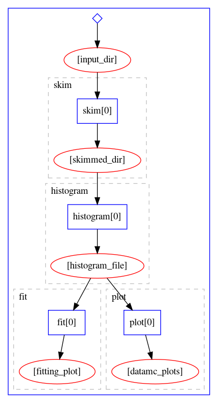
The workflow definition is similar to that of the Serial workflow created in the previous episode. As we can see, this already leads to certain parallelism, because the fitting stage and the plotting stage can actually run simultaneously once the histograms are produced. The graphical representation of the above workflow looks as follows:
Let us try to run it on REANA cloud.
Exercise
Write and run a HiggsToTauTau analysis example using the Yadage workflow version presented above. Take the workflow definition, the step definition, and write the corresponding
reana.yaml. Afterwards run the example on REANA cloud.
Solution
mkdir awesome-analysis-yadage-simple
cd awesome-analysis-yadage-simple
vim workflow.yaml # take workflow definition contents above
vim steps.yaml    # take step definition contents above
vim reana.yaml    # the goal of the exercise is to create this content
cat reana.yaml
inputs: files: - steps.yaml - workflow.yaml parameters: input_dir: root://eospublic.cern.ch//eos/root-eos/HiggsTauTauReduced workflow: type: yadage file: workflow.yaml
The Snakemake workflow can be expressed by the following Snakefile:
uri = "root://eospublic.cern.ch//eos/root-eos/HiggsTauTauReduced"

rule all:
    input:
        "fit/fit.png",
        "plot/pt_met.png"

rule skim:
    output:
        directory("skim")
    container:
        "docker://gitlab-registry.cern.ch/awesome-workshop/awesome-analysis-eventselection-stage3:master"
    shell:
        "workspace=$(pwd) && mkdir -p skim && cd /analysis/skim && bash ./skim.sh {uri} $workspace/skim"

rule histogram:
    input:
        "skim"
    output:
        "histogram/histograms.root"
    container:
        "docker://gitlab-registry.cern.ch/awesome-workshop/awesome-analysis-eventselection-stage3:master"
    shell:
        "workspace=$(pwd) && mkdir -p histogram && cd /analysis/skim && bash ./histograms_with_custom_output_location.sh $workspace/{input} $workspace/histogram"

rule fit:
    input:
        "histogram/histograms.root"
    output:
        "fit/fit.png"
    container:
        "docker://gitlab-registry.cern.ch/awesome-workshop/awesome-analysis-statistics-stage3:master"
    shell:
        "workspace=$(pwd) && mkdir -p fit && cd /fit && bash ./fit.sh $workspace/{input} $workspace/fit"

rule plot:
    input:
        "histogram/histograms.root"
    output:
        "plot/pt_met.png"
    container:
        "docker://gitlab-registry.cern.ch/awesome-workshop/awesome-analysis-eventselection-stage3:master"
    shell:
        "workspace=$(pwd) && mkdir -p plot && cd /analysis/skim && bash ./plot.sh $workspace/{input} $workspace/plot 0.1"
Let us try to run it on REANA cloud.
Exercise
Write and run a HiggsToTauTau analysis example using the Snakemake workflow version presented above. Take the workflow definition, the step definition, and write the corresponding
reana.yaml. Afterwards run the example on REANA cloud.
Solution
mkdir awesome-analysis-snakemake-simple
cd awesome-analysis-snakemake-simple
vim Snakefile     # take workflow definition contents above
vim reana.yaml    # the goal of the exercise is to create this content
cat reana.yaml
inputs: files: - Snakefile - reana.yaml workflow: type: snakemake file: Snakefile outputs: files: - fit/fit.png
Parallelism via scatter-gather paradigm
We have seen how to achieve a certain parallelism of workflow steps via simple dependency graph expressing which workflow steps depend on which others.
We now introduce a more advanced concept how to instruct the workflow engine to start many parallel computations. The paradigm is called “scatter-gather” and is used to instruct the workflow engine to run a certain parametrised command over an array of input values in parallel (the “scatter” operation) whilst assembling these results together afterwards (the “gather” operation). The “scatter-gather” paradigm allows to scale computations in a “map-reduce” fashion over input values with a minimal syntax without having to duplicate workflow code or write loop statements.
Here is an example of the scatter-gather paradigm in the Yadage language. Note the use of “multi-step” stage definition, expressing that the given stage is actually running multiple parametrised steps:
stages:
  - name: filter1
    dependencies: [init]
    scheduler:
      scheduler_type: multistep-stage
      parameters:
        input: {stages: init, output: input, unwrap: true}
      batchsize: 2
      scatter:
        method: zip
        parameters: [input]
      step: {$ref: steps.yaml#/filter}
  - name: filter2
    dependencies: [filter1]
    scheduler:
      scheduler_type: multistep-stage
      parameters:
        input: {stages: filter1, output: output, unwrap:true}
      batchsize: 2
      scatter:
        method: zip
        parameters: [input]
      step: {$ref: steps.yaml#/filter}
  - name: filter3
    dependencies: [filter2]
    scheduler:
      scheduler_type: singlestep-stage
      parameters:
        input: {stages: 'filter2', output: output}
      step: {$ref: steps.yaml#/filter}
The graphical representation of the computational graph looks like:
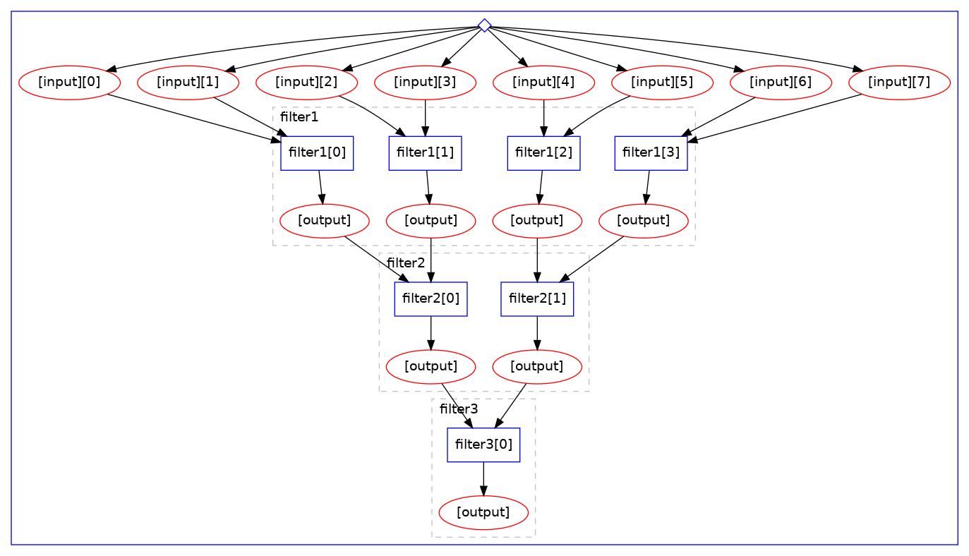
Note how the “scatter” operation is automatically happening over the given “input” array with the
wanted batch size, processing files two by two irrespective of the number of input files. Note
also the automatic “cascading” of computations.
Snakemake has several concepts how to parametrise calculations. One can start by using rule wildcards. For example, if we would like to process five data samples concurrently, you can specify rules like:
samples = ["1","2","3","4","5"]

rule scatter:
    input:
        "myinputs{n}.txt"
    output:
        "myresults{n}.txt"
    shell:
      ...

rule gather:
    input:
        expand("myresults{n}.txt", n=samples)
    output:
        "sum.txt"
    shell:
        ...
Here Snakemake will start five independent jobs to “scatter” computations over data, yielding
partial myresults.txt files for each sample, and then aggregates them as necessary in the “gather”
rule.
In the next episode we shall see how the scatter-gather paradigm can be used to speed up the HiggsToTauTau sequential workflow that we developed in the previous episode.
Key Points
Computational analysis is a graph of inter-dependent steps
Fully declare inputs and outputs for each step
Use dependencies between workflow steps to allow running jobs in parallel
Use scatter/gather paradigm to parallelise parametrised computations
HiggsToTauTau analysis: parallel
Overview
Teaching: 10 min
Exercises: 20 minQuestions
Challenge: write the HiggsToTauTau analysis parallel workflow and run it on REANA
Objectives
Develop a full HiggsToTauTau analysis workflow using parallel language
Overview
We have seen examples of full DAG-aware workflow languages (Snakemake and Yadage) and how they can be used to describe and run the RooFit example and a simple version of HiggsToTauTau example.
In this episode we shall see how to efficiently apply parallelism to speed up the HiggsToTauTau example via the scatter-gather paradigm introduced in the previous episode.
HiggsToTauTau analysis
Let us start by defining the overall skeleton of the analysis workflow.
The overall reana.yaml for this parallel analysis in Yadage looks like:
inputs:
  files:
    - steps.yaml
    - workflow.yaml
  parameters:
    files:
      - root://eospublic.cern.ch//eos/root-eos/HiggsTauTauReduced/GluGluToHToTauTau.root
      - root://eospublic.cern.ch//eos/root-eos/HiggsTauTauReduced/VBF_HToTauTau.root
      - root://eospublic.cern.ch//eos/root-eos/HiggsTauTauReduced/DYJetsToLL.root
      - root://eospublic.cern.ch//eos/root-eos/HiggsTauTauReduced/TTbar.root
      - root://eospublic.cern.ch//eos/root-eos/HiggsTauTauReduced/W1JetsToLNu.root
      - root://eospublic.cern.ch//eos/root-eos/HiggsTauTauReduced/W2JetsToLNu.root
      - root://eospublic.cern.ch//eos/root-eos/HiggsTauTauReduced/W3JetsToLNu.root
      - root://eospublic.cern.ch//eos/root-eos/HiggsTauTauReduced/Run2012B_TauPlusX.root
      - root://eospublic.cern.ch//eos/root-eos/HiggsTauTauReduced/Run2012C_TauPlusX.root
    cross_sections:
      - 19.6
      - 1.55
      - 3503.7
      - 225.2
      - 6381.2
      - 2039.8
      - 612.5
      - 1.0
      - 1.0
    short_hands:
      - [ggH]
      - [qqH]
      - [ZLL,ZTT]
      - [TT]
      - [W1J]
      - [W2J]
      - [W3J]
      - [dataRunB]
      - [dataRunC]
workflow:
  type: yadage
  file: workflow.yaml
outputs:
  files:
    - fit/fit.png
Note that the input files, cross-sections, and short names are defined as arrays. These are the arrays we will scatter over.
The overall reana.yaml for this parallel analysis in Snakemake looks like:
inputs:
  files:
    - Snakefile
workflow:
  type: snakemake
  file: Snakefile
outputs:
  files:
    - fit/fit.png
Note that this reana.yaml file is very minimal: we are basically only declaring that we shall use
Snakemake workflow type, and all the details will live in the Snakefile that will be defining the
workflow. The Snakefile will start by defining parameters:
uri = "root://eospublic.cern.ch//eos/root-eos/HiggsTauTauReduced"

files = [
    "GluGluToHToTauTau",
    "VBF_HToTauTau",
    "DYJetsToLL",
    "DYJetsToLL",
    "TTbar",
    "W1JetsToLNu",
    "W2JetsToLNu",
    "W3JetsToLNu",
    "Run2012B_TauPlusX",
    "Run2012C_TauPlusX",
]

cross_sections = [
    19.6,
    1.55,
    3503.7,
    3503.7,
    225.2,
    6381.2,
    2039.8,
    612.5,
    1.0,
    1.0,
]

short_hands = [
    "ggH",
    "qqH",
    "ZLL",
    "ZTT",
    "TT",
    "W1J",
    "W2J",
    "W3J",
    "dataRunB",
    "dataRunC",
]
Note how we have defined files, cross_sections, and short_hands representing various data
sets that we shall be processing in parallel. We shall use these arrays as Snakemake wildcards
over which the computations will be distributed in a parallel manner. The short_hands array
gives each dataset a compact label used in downstream rules and output filenames.
Note also that DYJetsToLL appears twice on purpose: the same input dataset is processed under
two different selections, ZLL (Z → ℓℓ) and ZTT (Z → ττ). Because Snakemake aligns the three
arrays element-by-element, the file and its cross-section are repeated so that each selection
gets its own scatter slot.
We can also declare the desired overall final outputs of the workflow:
rule all:
    input:
        "fit/fit.png",
        "plot/pt_met.png"
The rest of the Snakefile will be discussed below.
HiggsToTauTau skimming
The skimming step definition looks like:
- name: skim
  dependencies: [init]
  scheduler:
    scheduler_type: multistep-stage
    parameters:
      input_file: {step: init, output: files}
      cross_section: {step: init, output: cross_sections}
      output_file: '{workdir}/skimmed.root'
    scatter:
       method: zip
       parameters: [input_file, cross_section]
    step: {$ref: 'steps.yaml#/skim'}
where the step is defined as:
skim:
  process:
    process_type: 'interpolated-script-cmd'
    script: |
      ./skim {input_file} {output_file} {cross_section} 11467.0 0.1
  environment:
    environment_type: 'docker-encapsulated'
    image: gitlab-registry.cern.ch/awesome-workshop/awesome-analysis-eventselection-stage3
    imagetag: master
  publisher:
    publisher_type: interpolated-pub
    publish:
      skimmed_file: '{output_file}'
Note the scatter paradigm that will cause nine parallel jobs for each input dataset file.
rule skim:
    output:
        "skim/{files}_{cross_sections}.root"
    container:
        "docker://gitlab-registry.cern.ch/awesome-workshop/awesome-analysis-eventselection-stage3:master"
    shell:
        "workspace=$(pwd) && mkdir -p skim && cd /analysis/skim && ./skim {uri}/{wildcards.files}.root $workspace/{output} {wildcards.cross_sections} 11467.0 0.1"
HiggsToTauTau histogramming
The histograms can be produced as follows:
- name: histogram
  dependencies: [skim]
  scheduler:
    scheduler_type: multistep-stage
    parameters:
      input_file: {stages: skim, output: skimmed_file}
      output_names: {step: init, output: short_hands}
      output_dir: '{workdir}'
    scatter:
       method: zip
       parameters: [input_file, output_names]
    step: {$ref: 'steps.yaml#/histogram'}
with:
histogram:
  process:
    process_type: 'interpolated-script-cmd'
    script: |
      for x in {output_names}; do
        python histograms.py {input_file} $x {output_dir}/$x.root;
      done
  environment:
    environment_type: 'docker-encapsulated'
    image: gitlab-registry.cern.ch/awesome-workshop/awesome-analysis-eventselection-stage3
    imagetag: master
  publisher:
    publisher_type: interpolated-pub
    glob: true
    publish:
      histogram_file: '{output_dir}/*.root'
rule histogram:
    input:
        "skim/{files}_{cross_sections}.root"
    output:
        "histogram/{files}_{cross_sections}_{short_hands}.root"
    container:
        "docker://gitlab-registry.cern.ch/awesome-workshop/awesome-analysis-eventselection-stage3:master"
    shell:
        "workspace=$(pwd) && mkdir -p histogram && cd /analysis/skim && python histograms.py $workspace/{input} {wildcards.short_hands} $workspace/{output}"
HiggsToTauTau merging
Time to gather! How do we merge scattered results?
- name: merge
  dependencies: [histogram]
  scheduler:
    scheduler_type: singlestep-stage
    parameters:
      input_files: {stages: histogram, output: histogram_file, flatten: true}
      output_file: '{workdir}/merged.root'
    step: {$ref: 'steps.yaml#/merge'}
with:
merge:
  process:
    process_type: 'interpolated-script-cmd'
    script: |
      hadd {output_file} {input_files}
  environment:
    environment_type: 'docker-encapsulated'
    image: gitlab-registry.cern.ch/awesome-workshop/awesome-analysis-eventselection-stage3
    imagetag: master
  publisher:
    publisher_type: interpolated-pub
    publish:
      merged_file: '{output_file}'
rule merge:
    input:
        expand("histogram/{files}_{cross_sections}_{short_hands}.root", zip, files=files, cross_sections=cross_sections, short_hands=short_hands)
    output:
        "merge/merged.root"
    container:
        "docker://gitlab-registry.cern.ch/awesome-workshop/awesome-analysis-eventselection-stage3:master"
    shell:
        "mkdir -p merge && hadd {output} {input}"
HiggsToTauTau fitting
The fit can be performed as follows:
- name: fit
  dependencies: [merge]
  scheduler:
    scheduler_type: singlestep-stage
    parameters:
      histogram_file: {step: merge, output: merged_file}
      fit_outputs: '{workdir}'
    step: {$ref: 'steps.yaml#/fit'}
with:
fit:
  process:
    process_type: 'interpolated-script-cmd'
    script: |
      python fit.py {histogram_file} {fit_outputs}
  environment:
    environment_type: 'docker-encapsulated'
    image: gitlab-registry.cern.ch/awesome-workshop/awesome-analysis-statistics-stage3
    imagetag: master
  publisher:
    publisher_type: interpolated-pub
    publish:
      fit_results: '{fit_outputs}/fit.png'
rule fit:
    input:
        "merge/merged.root"
    output:
        "fit/fit.png"
    container:
        "docker://gitlab-registry.cern.ch/awesome-workshop/awesome-analysis-statistics-stage3:master"
    shell:
        "workspace=$(pwd) && mkdir -p fit && cd /fit && python fit.py $workspace/{input} $workspace/fit"
HiggsToTauTau plotting
Challenge time! Add plotting step to the workflow.
Exercise
Following the example above, write plotting step and plug it into the overall workflow.
Solution
The addition to the workflow specification is:
- name: plot
  dependencies: [merge]
  scheduler:
    scheduler_type: singlestep-stage
    parameters:
      histogram_file: {step: merge, output: merged_file}
      plot_outputs: '{workdir}'
    step: {$ref: 'steps.yaml#/plot'}
The step is being defined as:
plot:
  process:
    process_type: 'interpolated-script-cmd'
    script: |
      python plot.py {histogram_file} {plot_outputs} 0.1
  environment:
    environment_type: 'docker-encapsulated'
    image: gitlab-registry.cern.ch/awesome-workshop/awesome-analysis-eventselection-stage3
    imagetag: master
  publisher:
    publisher_type: interpolated-pub
    publish:
      fitting_plot: '{plot_outputs}'
rule plot:
    input:
        "merge/merged.root"
    output:
        "plot/pt_met.png"
    container:
        "docker://gitlab-registry.cern.ch/awesome-workshop/awesome-analysis-eventselection-stage3:master"
    shell:
        "workspace=$(pwd) && mkdir -p plot && cd /analysis/skim && python plot.py $workspace/{input} $workspace/plot 0.1"
Full workflow
We are now ready to assemble the previous stages together and run the example on the REANA cloud.
Exercise
Write and run the HiggsToTauTau parallel workflow on REANA cloud. How many jobs does the workflow have? How much faster is it executed compared to the simple serial version?
Solution
The REANA specification file reana.yaml looks as follows:
inputs:
  files:
    - steps.yaml
    - workflow.yaml
  parameters:
    files:
      - root://eospublic.cern.ch//eos/root-eos/HiggsTauTauReduced/GluGluToHToTauTau.root
      - root://eospublic.cern.ch//eos/root-eos/HiggsTauTauReduced/VBF_HToTauTau.root
      - root://eospublic.cern.ch//eos/root-eos/HiggsTauTauReduced/DYJetsToLL.root
      - root://eospublic.cern.ch//eos/root-eos/HiggsTauTauReduced/TTbar.root
      - root://eospublic.cern.ch//eos/root-eos/HiggsTauTauReduced/W1JetsToLNu.root
      - root://eospublic.cern.ch//eos/root-eos/HiggsTauTauReduced/W2JetsToLNu.root
      - root://eospublic.cern.ch//eos/root-eos/HiggsTauTauReduced/W3JetsToLNu.root
      - root://eospublic.cern.ch//eos/root-eos/HiggsTauTauReduced/Run2012B_TauPlusX.root
      - root://eospublic.cern.ch//eos/root-eos/HiggsTauTauReduced/Run2012C_TauPlusX.root
    cross_sections:
      - 19.6
      - 1.55
      - 3503.7
      - 225.2
      - 6381.2
      - 2039.8
      - 612.5
      - 1.0
      - 1.0
    short_hands:
      - [ggH]
      - [qqH]
      - [ZLL, ZTT]
      - [TT]
      - [W1J]
      - [W2J]
      - [W3J]
      - [dataRunB]
      - [dataRunC]
workflow:
  type: yadage
  file: workflow.yaml
outputs:
  files:
    - fit/fit.png
The workflow definition file workflow.yaml is:
stages:
- name: skim
  dependencies: [init]
  scheduler:
    scheduler_type: multistep-stage
    parameters:
      input_file: {step: init, output: files}
      cross_section: {step: init, output: cross_sections}
      output_file: '{workdir}/skimmed.root'
    scatter:
       method: zip
       parameters: [input_file, cross_section]
    step: {$ref: 'steps.yaml#/skim'}

- name: histogram
  dependencies: [skim]
  scheduler:
    scheduler_type: multistep-stage
    parameters:
      input_file: {stages: skim, output: skimmed_file}
      output_names: {step: init, output: short_hands}
      output_dir: '{workdir}'
    scatter:
       method: zip
       parameters: [input_file, output_names]
    step: {$ref: 'steps.yaml#/histogram'}

- name: merge
  dependencies: [histogram]
  scheduler:
    scheduler_type: singlestep-stage
    parameters:
      input_files: {stages: histogram, output: histogram_file, flatten: true}
      output_file: '{workdir}/merged.root'
    step: {$ref: 'steps.yaml#/merge'}

- name: fit
  dependencies: [merge]
  scheduler:
    scheduler_type: singlestep-stage
    parameters:
      histogram_file: {step: merge, output: merged_file}
      fit_outputs: '{workdir}'
    step: {$ref: 'steps.yaml#/fit'}

- name: plot
  dependencies: [merge]
  scheduler:
    scheduler_type: singlestep-stage
    parameters:
      histogram_file: {step: merge, output: merged_file}
      plot_outputs: '{workdir}'
    step: {$ref: 'steps.yaml#/plot'}
The workflow steps defined in steps.yaml are:
skim:
  process:
    process_type: 'interpolated-script-cmd'
    script: |
      ./skim {input_file} {output_file} {cross_section} 11467.0 0.1
  environment:
    environment_type: 'docker-encapsulated'
    image: gitlab-registry.cern.ch/awesome-workshop/awesome-analysis-eventselection-stage3
    imagetag: master
  publisher:
    publisher_type: interpolated-pub
    publish:
      skimmed_file: '{output_file}'

histogram:
  process:
    process_type: 'interpolated-script-cmd'
    script: |
      for x in {output_names}; do
        python histograms.py {input_file} $x {output_dir}/$x.root;
      done
  environment:
    environment_type: 'docker-encapsulated'
    image: gitlab-registry.cern.ch/awesome-workshop/awesome-analysis-eventselection-stage3
    imagetag: master
  publisher:
    publisher_type: interpolated-pub
    glob: true
    publish:
      histogram_file: '{output_dir}/*.root'

merge:
  process:
    process_type: 'interpolated-script-cmd'
    script: |
      hadd {output_file} {input_files}
  environment:
    environment_type: 'docker-encapsulated'
    image: gitlab-registry.cern.ch/awesome-workshop/awesome-analysis-eventselection-stage3
    imagetag: master
  publisher:
    publisher_type: interpolated-pub
    publish:
      merged_file: '{output_file}'

fit:
  process:
    process_type: 'interpolated-script-cmd'
    script: |
      python fit.py {histogram_file} {fit_outputs}
  environment:
    environment_type: 'docker-encapsulated'
    image: gitlab-registry.cern.ch/awesome-workshop/awesome-analysis-statistics-stage3
    imagetag: master
  publisher:
    publisher_type: interpolated-pub
    publish:
      fit_results: '{fit_outputs}/fit.png'

plot:
  process:
    process_type: 'interpolated-script-cmd'
    script: |
      python plot.py {histogram_file} {plot_outputs} 0.1
  environment:
    environment_type: 'docker-encapsulated'
    image: gitlab-registry.cern.ch/awesome-workshop/awesome-analysis-eventselection-stage3
    imagetag: master
  publisher:
    publisher_type: interpolated-pub
    publish:
      fitting_plot: '{plot_outputs}'
The REANA specification file reana.yaml looks as follows:
inputs:
  files:
    - Snakefile
workflow:
  type: snakemake
  file: Snakefile
outputs:
  files:
    - fit/fit.png
The workflow definition file Snakefile is:
uri = "root://eospublic.cern.ch//eos/root-eos/HiggsTauTauReduced"

files = [
    "GluGluToHToTauTau",
    "VBF_HToTauTau",
    "DYJetsToLL",
    "DYJetsToLL",
    "TTbar",
    "W1JetsToLNu",
    "W2JetsToLNu",
    "W3JetsToLNu",
    "Run2012B_TauPlusX",
    "Run2012C_TauPlusX",
]

cross_sections = [
    19.6,
    1.55,
    3503.7,
    3503.7,
    225.2,
    6381.2,
    2039.8,
    612.5,
    1.0,
    1.0,
]

short_hands = [
    "ggH",
    "qqH",
    "ZLL",
    "ZTT",
    "TT",
    "W1J",
    "W2J",
    "W3J",
    "dataRunB",
    "dataRunC",
]

rule all:
    input:
        "fit/fit.png",
        "plot/pt_met.png"

rule skim:
    output:
        "skim/{files}_{cross_sections}.root"
    container:
        "docker://gitlab-registry.cern.ch/awesome-workshop/awesome-analysis-eventselection-stage3:master"
    shell:
        "workspace=$(pwd) && mkdir -p skim && cd /analysis/skim && ./skim {uri}/{wildcards.files}.root $workspace/{output} {wildcards.cross_sections} 11467.0 0.1"

rule histogram:
    input:
        "skim/{files}_{cross_sections}.root"
    output:
        "histogram/{files}_{cross_sections}_{short_hands}.root"
    container:
        "docker://gitlab-registry.cern.ch/awesome-workshop/awesome-analysis-eventselection-stage3:master"
    shell:
        "workspace=$(pwd) && mkdir -p histogram && cd /analysis/skim && python histograms.py $workspace/{input} {wildcards.short_hands} $workspace/{output}"

rule merge:
    input:
        expand("histogram/{files}_{cross_sections}_{short_hands}.root", zip, files=files, cross_sections=cross_sections, short_hands=short_hands)
    output:
        "merge/merged.root"
    container:
        "docker://gitlab-registry.cern.ch/awesome-workshop/awesome-analysis-eventselection-stage3:master"
    shell:
        "mkdir -p merge && hadd {output} {input}"

rule fit:
    input:
        "merge/merged.root"
    output:
        "fit/fit.png"
    container:
        "docker://gitlab-registry.cern.ch/awesome-workshop/awesome-analysis-statistics-stage3:master"
    shell:
        "workspace=$(pwd) && mkdir -p fit && cd /fit && python fit.py $workspace/{input} $workspace/fit"

rule plot:
    input:
        "merge/merged.root"
    output:
        "plot/pt_met.png"
    container:
        "docker://gitlab-registry.cern.ch/awesome-workshop/awesome-analysis-eventselection-stage3:master"
    shell:
        "workspace=$(pwd) && mkdir -p plot && cd /analysis/skim && python plot.py $workspace/{input} $workspace/plot 0.1"
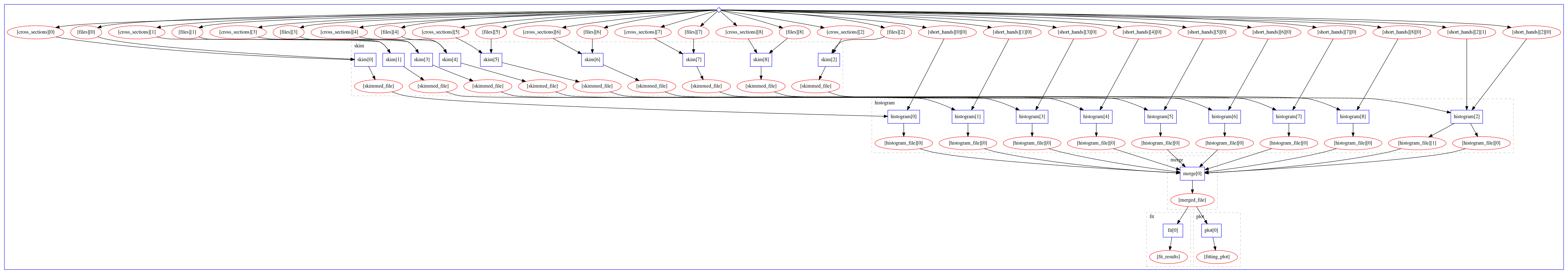
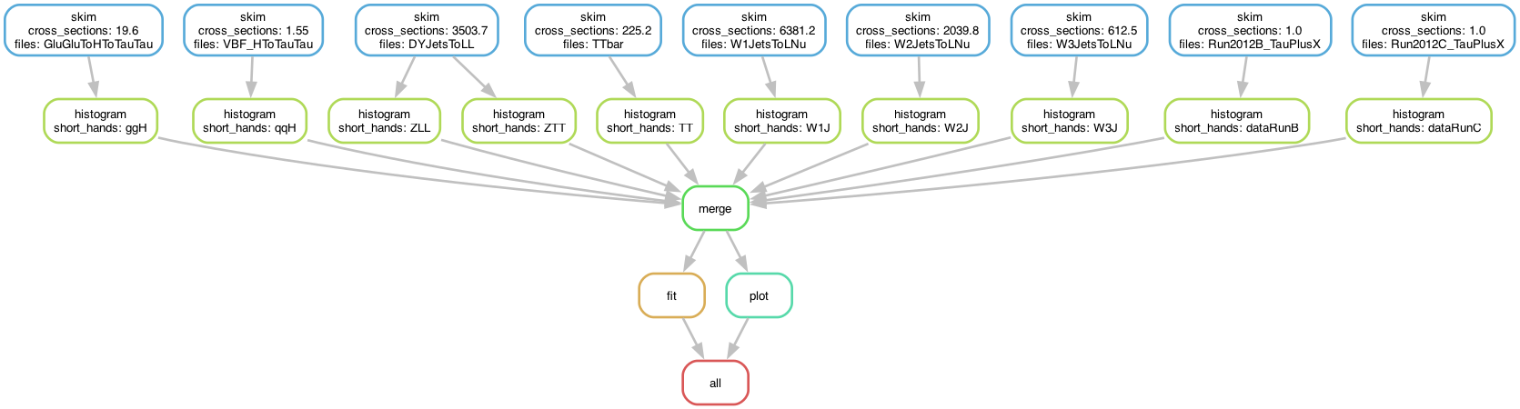
Results
The computational graph of the workflow looks like:
The workflow produces the following fit:

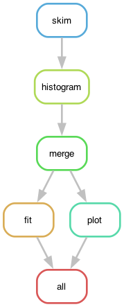
The dependency graph of the workflow rules, defined in Snakefile, looks like:
The skimming and histogramming calculations were parallelised over various input files, leading to the following runtime computational graph:
The workflow produces the following fit:
Key Points
Use step dependencies to express main analysis stages
Use scatter-gather paradigm in stages to massively parallelise DAG workflow execution
REANA usage scenarios remain the same regardless of workflow language details
A glimpse on advanced topics
Overview
Teaching: 15 min
Exercises: 5 minQuestions
Can I publish workflow results on EOS?
Can I use Kerberos to access restricted resources?
Can I use CVMFS software repositories?
Can I dispatch heavy computations to HTCondor?
Can I dispatch heavy computations to Slurm?
Can I open Jupyter notebooks on my REANA workspace?
Can I connect my GitLab repositories with REANA?
Objectives
Learn about advanced possibilities of REANA platform
Learn how to use Kerberos secrets to access restricted resources
Learn how to interact with remote storage solutions (EOS)
Learn how to interact with remote compute backends (HTCondor, Slurm)
Learn how to interact with remote code repositories (CVMFS, GitLab)
Learn how to open interactive sessions (Jupyter notebooks)
Overview
We now know how to write serial and parallel workflows.
What do we need more in order to use the system for real life physics analyses?
Let’s scratch the surface of some more advanced topics:
- Publishing workflow artifacts on EOS
- Using CVMFS software repositories
- Using high-throughput computing backends: HTCondor
- Using high-performance computing backends: Slurm
- Opening interactive environments (notebooks) on workflow workspace
- Bridging GitLab with REANA
Publishing workflow results on EOS
REANA uses shared filesystem for storing results of your running workflows. They may be
garbage-collected after a certain period of time. You can use the reana-client download command
to download the results of your workflows, as we have seen in Episode 2. Is there a more automatic
way?
One possibility is to add a final step to your workflow that would publish the results of interest in outside filesystem. For example, how can you publish all resulting plots in your personal EOS folder?
First, you have to let the REANA platform know your Kerberos keytab so that writing to EOS would be authorised.
If you don’t have a keytab file yet, you can generate it on LXPLUS by using the following command
(assuming the user login name to be johndoe):
cern-get-keytab --keytab ~/.keytab --user --login johndoe
Check whether it works:
kdestroy; kinit -kt ~/.keytab johndoe; klist
Ticket cache: FILE:/tmp/krb5cc_1234_5678
Default principal: johndoe@CERN.CH

Valid starting       Expires              Service principal
07/05/2023 18:04:13  07/06/2023 19:04:13  krbtgt/CERN.CH@CERN.CH
    renew until 07/10/2023 18:04:13
07/05/2023 18:04:13  07/06/2023 19:04:13  afs/cern.ch@CERN.CH
    renew until 07/10/2023 18:04:13
Upload it to the REANA platform as “user secrets”:
reana-client secrets-add --env CERN_USER=johndoe \
                         --env CERN_KEYTAB=.keytab \
                         --file ~/.keytab
Second, once your Kerberos user secrets are uploaded to the REANA platform, you can modify your workflow to add a final data publishing step that copies the resulting plots to the desired EOS directories:
workflow:
  type: serial
  specification:
    steps:
      - name: myfirststep
        ...
      - name: mysecondstep
        ...
      - name: publish
        environment: 'docker.io/library/ubuntu:20.04'
        kerberos: true
        kubernetes_memory_limit: '256Mi'
        commands:
          - mkdir -p /eos/home-j/johndoe/myanalysis-outputs
          - cp myplots/*.png /eos/home-j/johndoe/myanalysis-outputs/
Note the presence of the kerberos: true clause in the final publishing step definition which
instructs the REANA system to initialise the Kerberos-based authentication process using the
provided user secrets.
Exercise
Publish some of the produced HigssToTauTau analysis plots to your EOS home directory.
Solution
Modify your workflow specification to add a final publishing step.
Hint: Use a previously finished analysis run and the
restartcommand so that you don’t have to rerun the full analysis again.If you need more assistance with creating and uploading keytab files, please see the REANA documentation on Keytab.
If you need more assistance with creating final workflow publishing step, please see the REANA documentation on EOS.
Using CVMFS software repositories
Many physics analyses need software living in CVMFS filesystem. Packaging this software into the container is possible, but it could make the container size enormous. Can we access CVMFS filesystem at runtime?
REANA allows to specify custom resource need declarations in reana.yaml by means of a
resources clause. An example:
workflow:
  type: serial
  resources:
    cvmfs:
      - fcc.cern.ch
  specification:
    steps:
      - environment: 'docker.io/cern/slc6-base'
        commands:
        - ls -l /cvmfs/fcc.cern.ch/sw/views/releases/
Exercise
Write a workflow that would run ROOT from the SFT repository on CVMFS and that would list all configuration flags enabled in that executable.
Solution
See also REANA documentation on CVMFS.
Using high-throughput computing backends: HTCondor
REANA uses Kerberos as its default compute backend.
Massively parallel physics analyses profit from HTC computing systems such as HTCondor to launch same procedures on mutually independent data files.
If you would like to dispatch parts of the workflow to HTCondor backend, you can use the
compute_backend clause of the workflow specification, for example:
workflow:
  type: serial
  specification:
    steps:
      - name: gendata
        environment: 'docker.io/reanahub/reana-env-root6:6.18.04'
        compute_backend: htcondorcern
        htcondor_max_runtime: espresso
        commands:
        - mkdir -p results && root -b -q 'code/gendata.C(${events},"${data}")'
Note that the access control will be handled automatically via Kerberos, so this requires you to
submit your keytab as in the EOS publishing example above.
Exercise
Modify HiggsToTauTau analysis to run the skimming part on the HTCondor cluster.
Solution
See also REANA documentation on HTCondor.
Using high-performance computing backends: Slurm
Another useful compute backend architecture is HPC with inter-connected nodes. This is useful for MPI and similar programming techniques.
REANA supports Slurm job scheduler to send jobs to HPC clusters. You can simply use the
compute_backend clause again to specify wanted compute backend for each step:
workflow:
  type: serial
  specification:
    steps:
      - name: gendata
        environment: 'docker.io/reanahub/reana-env-root6:6.18.04'
        compute_backend: slurmcern
        commands:
        - mkdir -p results && root -b -q 'code/gendata.C(${events},"${data}")'
Exercise
Modify HiggsToTauTau analysis to run the histogramming part on the Slurm cluster.
Solution
See also REANA documentation on Slurm.
Opening interactive environments (notebooks) on workflow workspace
While your analysis workflows are running, you may want to open interactive session processes on the
workflow workspace. For example, to run a Jupyter notebook. This can be achieved via the open
command:
reana-client open -w myanalysis.42
The command will generate unique URL that will become active after a minute or two and where you will be able to open a notebook or a remote terminal on your workflow workspace.
When the notebook is no longer needed, it can be brought down via the close command:
reana-client close -w myanalysis.42
Exercise
Open a Jupyter notebook on your HiggsToTauTau analysis example and inspect the ROOT files there.
Solution
See also REANA documentation on running notebooks.
Bridging GitLab with REANA
When using GitLab for source code development, GitLab’s native Continuous Integration runners offer a comfortable testing environment for your analyses.
However, the CPU time is usually limited.
If you would like to run REANA workflows directly from GitLab, it is useful to bridge the REANA platform and GitLab via OAuth technology.
This can be easily achieved from “Your profile” page on REANA user interface:
firefox https://reana.cern.ch/
Exercise
Connect your REANA account and your GitLab account and run an example analysis from GitLab on REANA cloud.
Solution
Key Points
Workflow specification uses hints to hide implementation complexity
Use
kerberos: trueclause to automatically trigger Kerberos token initialisationUse
resourcesclause to access CVMFS repositoriesUse
compute_backendhint in your workflow steps to dispatch jobs to various HPC/HTC backendsUse
open/closecommands to open and close interactive sessions on your workspaceEnable REANA application on GitLab to run long-standing tasks that would time out in GitLab CI
Wrap-up
Overview
Teaching: 5 min
Exercises: 0 minQuestions
What have we learned today?
Where to go from here?
Objectives
Learn about REANA community
Wrapping up
We have discussed the problem of reproducibility and reusability of scientific analyses.
We have practiced the declarative programming approach through several examples of containerised scientific workflows.
We have seen some of the capabilities of the REANA platform allowing you to easily run containerised scientific workflows on remote compute clouds.
Please experiment with the containerised scientific workflows and let us know what you think!
The REANA platform is in a pilot stage; the early feedback with real-life use cases is greatly appreciated.
Get in touch:
- Discuss on Forum
- Chat on Mattermost
- Follow us on Twitter
- Collaborate on GitHub
Thanks and here’s to many preproducible analyses ;)
Key Points
Experiment with containerised workflows to advance scientific reproducibility in your research