Developing parallel workflows
Overview
Teaching: 15 min
Exercises: 10 minQuestions
How to scale up and run thousands of jobs?
What is a DAG?
What is a Scatter-Gather paradigm?
How to run Yadage workflows on REANA?
Objectives
Learn about Directed Acyclic Graphs (DAG)
Understand Yadage workflow language
Practice running and inspecting parallel workflows
Overview
We now know how to develop reproducible analyses on small scale using serial workflows.
In this lesson we shall learn how to scale up for real-life work which usually requires using parallel workflows.
Computational workflows as Directed Acyclic Graphs (DAG)
Computational workflows can be expressed as a set of computational steps where some steps depend on other steps before they can begin their computations. In other words, the computational steps constitute a Directed Acyclic Graph (DAG) where each graph vertex represents a unit of computation with its inputs and outputs, and the graph edges describe the interconnections between computational steps. For example:
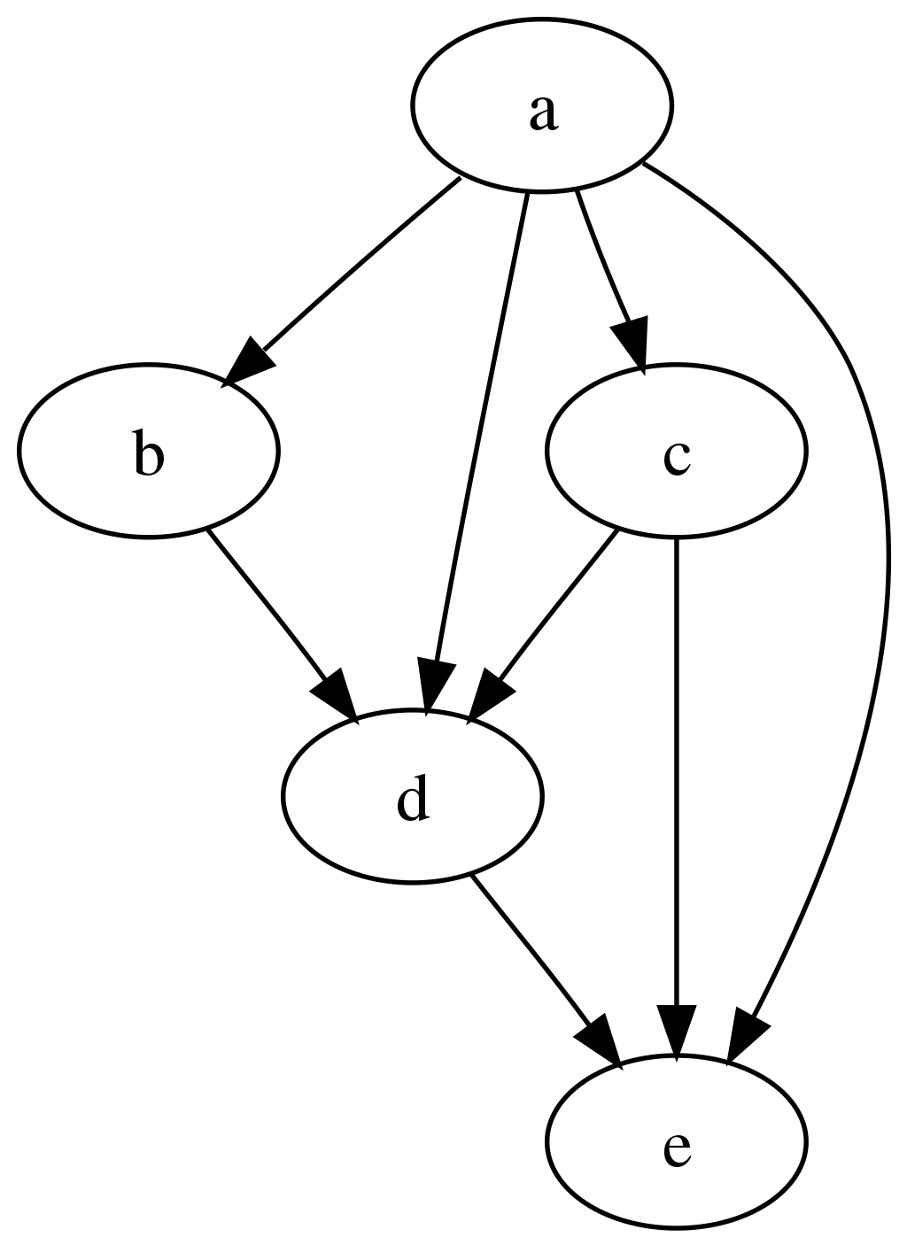
The graph is “directed” and “acyclic” because it can be topologically ordered so that later steps depend on earlier steps without cyclic dependencies, with progress flowing steadily from earlier steps to later steps.
The REANA platform supports several DAG workflow specification languages:
- Common Workflow Language (CWL) originated in life sciences;
- Snakemake originated in bioinformatics;
- Yadage originated in particle physics.
Workflow specification languages
The examples in this lesson use Snakemake (used e.g. in LHCb) and Yadage (used e.g. in ATLAS). Select a tab below to see the RooFit example expressed in each language.
Yadage enables describing even very complex computational workflows. Here is the Yadage specification for the RooFit example used in the previous episodes:
stages:
  - name: gendata
    dependencies: [init]
    scheduler:
      scheduler_type: 'singlestep-stage'
      parameters:
        events: {step: init, output: events}
        gendata: {step: init, output: gendata}
        outfilename: '{workdir}/data.root'
      step:
        process:
          process_type: 'interpolated-script-cmd'
          script: root -b -q '{gendata}({events},"{outfilename}")'
        publisher:
          publisher_type: 'frompar-pub'
          outputmap:
            data: outfilename
        environment:
          environment_type: 'docker-encapsulated'
          image: 'docker.io/reanahub/reana-env-root6'
          imagetag: '6.18.04'
  - name: fitdata
    dependencies: [gendata]
    scheduler:
      scheduler_type: 'singlestep-stage'
      parameters:
        fitdata: {step: init, output: fitdata}
        data: {step: gendata, output: data}
        outfile: '{workdir}/plot.png'
      step:
        process:
          process_type: 'interpolated-script-cmd'
          script: root -b -q '{fitdata}("{data}","{outfile}")'
        publisher:
          publisher_type: 'frompar-pub'
          outputmap:
            plot: outfile
        environment:
          environment_type: 'docker-encapsulated'
          image: 'docker.io/reanahub/reana-env-root6'
          imagetag: '6.18.04'
We can see that the workflow consists of two stages, the gendata stage that does not depend on
anything (this is denoted by [init] dependency which means the stage can run right after the
workflow initialisation already), and the fitdata stage that depends on the completion of the
gendata stage (this is denoted by [gendata]).
Note that each stage consists of a single workflow step (singlestep-stage) which represents the
basic unit of computation of the workflow. (We shall see below an example of a multi-step stages
which express the same basic unit of computations scattered over inputs.)
The step consists of the description of the process to run, the containerised environment in which to run the process, as well as the mapping of its outputs to the stage.
This is how the Yadage workflow engine understands which stages can be run in which order, what commands to run in each stage, and how to pass inputs and outputs between steps.
Snakemake uses “rules” where each rule defines its inputs and outputs and the command to run to produce them. The Snakemake workflow engine then computes the dependencies between rules based on how the outputs from some rules are used as inputs to other rules.
rule all:
    input:
        "results/data.root",
        "results/plot.png"

rule gendata:
    output:
        "results/data.root"
    params:
        events=20000
    container:
        "docker://docker.io/reanahub/reana-env-root6:6.18.04"
    shell:
        "mkdir -p results && root -b -q 'code/gendata.C({params.events},\"{output}\")'"

rule fitdata:
    input:
        data="results/data.root"
    output:
        "results/plot.png"
    container:
        "docker://docker.io/reanahub/reana-env-root6:6.18.04"
    shell:
        "root -b -q 'code/fitdata.C(\"{input.data}\",\"{output}\")'"
We see that the final plot is produced by the “fitdata” rule, which needs “data.root” file to be
present, and it is the “gendata” rule that produces it. Hence Snakemake knows that it has to run
the “gendata” rule first, and the computation of “fitdata” is deferred until “gendata” successfully
completes. This process is very similar to how Makefile are being used in Unix software packages.
Running on REANA
We have to instruct REANA which workflow engine to use by editing reana.yaml. Select a tab
below to see the configuration for each engine.
inputs:
  files:
    - code/gendata.C
    - code/fitdata.C
    - workflow.yaml
  parameters:
    events: 20000
    gendata: code/gendata.C
    fitdata: code/fitdata.C
workflow:
  type: yadage
  file: workflow.yaml
outputs:
  files:
    - results/plot.png
Here, workflow.yaml is a new file with the same content as specified above.
Exercise
Run RooFit example using Yadage workflow engine on the REANA cloud. Upload code, run workflow, inspect status, check logs, download final plot.
Solution
Nothing changes in the usual user interaction with the REANA platform:
reana-client create -w my-workflow -f ./reana.yaml
reana-client upload ./code -w my-workflow
reana-client start -w my-workflow
reana-client status -w my-workflow
reana-client logs -w my-workflow
reana-client ls -w my-workflow
reana-client download results/plot.png -w my-workflow
inputs:
  files:
    - code/gendata.C
    - code/fitdata.C
    - Snakefile
workflow:
  type: snakemake
  file: Snakefile
outputs:
  files:
    - results/plot.png
Here, Snakefile is a new file with the same content as specified above.
Exercise
Run RooFit example using Snakemake workflow engine on the REANA cloud. Upload code, run workflow, inspect status, check logs, download final plot.
Solution
Nothing changes in the usual user interaction with the REANA platform:
reana-client create -w my-workflow -f ./reana.yaml
reana-client upload ./code -w my-workflow
reana-client start -w my-workflow
reana-client status -w my-workflow
reana-client logs -w my-workflow
reana-client ls -w my-workflow
reana-client download results/plot.png -w my-workflow
Physics code vs orchestration code
Note that it wasn’t necessary to change anything in our research code: we simply modified the workflow definition and could run the RooFit code “as is” using a different workflow engine. This is a simple demonstration of the separation of concerns between “physics code” and “orchestration code”.
Parallelism via step dependencies
We have seen how the sequential workflows were expressed in the Snakemake/Yadage syntax using stage dependencies. Note that if the stage dependency graph would have permitted, the workflow steps not depending on each other, or on the results of previous computations, would have been executed in parallel by the workflow engine out of the box. The physicist only needs to specify which steps depend on which others, and the workflow engine takes care of efficiently starting and scheduling tasks as necessary.
HiggsToTauTau analysis: simple version
Let us demonstrate how to write a workflow for the HiggsToTauTau example analysis using simple step dependencies. Select a tab below to see the workflow expressed in each language.
The workflow stages look like:
stages:
- name: skim
  dependencies: [init]
  scheduler:
    scheduler_type: singlestep-stage
    parameters:
      input_dir: {step: init, output: input_dir}
      output_dir: '{workdir}/output'
    step: {$ref: 'steps.yaml#/skim'}

- name: histogram
  dependencies: [skim]
  scheduler:
    scheduler_type: singlestep-stage
    parameters:
      input_dir: {step: skim, output: skimmed_dir}
      output_dir: '{workdir}/output'
    step: {$ref: 'steps.yaml#/histogram'}

- name: fit
  dependencies: [histogram]
  scheduler:
    scheduler_type: singlestep-stage
    parameters:
      histogram_file: {step: histogram, output: histogram_file}
      output_dir: '{workdir}/output'
    step: {$ref: 'steps.yaml#/fit'}

- name: plot
  dependencies: [histogram]
  scheduler:
    scheduler_type: singlestep-stage
    parameters:
      histogram_file: {step: histogram, output: histogram_file}
      output_dir: '{workdir}/output'
    step: {$ref: 'steps.yaml#/plot'}
where steps are expressed as:
skim:
  process:
    process_type: 'interpolated-script-cmd'
    script: |
      mkdir {output_dir}
      bash skim.sh {input_dir} {output_dir}
  environment:
    environment_type: 'docker-encapsulated'
    image: gitlab-registry.cern.ch/awesome-workshop/awesome-analysis-eventselection-stage3
    imagetag: master
  publisher:
    publisher_type: interpolated-pub
    publish:
      skimmed_dir: '{output_dir}'

histogram:
  process:
    process_type: 'interpolated-script-cmd'
    script: |
      mkdir {output_dir}
      bash histograms_with_custom_output_location.sh {input_dir} {output_dir}
  environment:
    environment_type: 'docker-encapsulated'
    image: gitlab-registry.cern.ch/awesome-workshop/awesome-analysis-eventselection-stage3
    imagetag: master
  publisher:
    publisher_type: interpolated-pub
    publish:
      histogram_file: '{output_dir}/histograms.root'

plot:
  process:
    process_type: 'interpolated-script-cmd'
    script: |
      mkdir {output_dir}
      bash plot.sh {histogram_file} {output_dir}
  environment:
    environment_type: 'docker-encapsulated'
    image: gitlab-registry.cern.ch/awesome-workshop/awesome-analysis-eventselection-stage3
    imagetag: master
  publisher:
    publisher_type: interpolated-pub
    publish:
      datamc_plots: '{output_dir}'

fit:
  process:
    process_type: 'interpolated-script-cmd'
    script: |
      mkdir {output_dir}
      bash fit.sh {histogram_file} {output_dir}
  environment:
    environment_type: 'docker-encapsulated'
    image: gitlab-registry.cern.ch/awesome-workshop/awesome-analysis-statistics-stage3
    imagetag: master
  publisher:
    publisher_type: interpolated-pub
    publish:
      fitting_plot: '{output_dir}/fit.png'
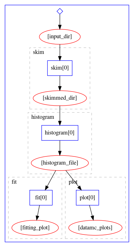
The workflow definition is similar to that of the Serial workflow created in the previous episode. As we can see, this already leads to certain parallelism, because the fitting stage and the plotting stage can actually run simultaneously once the histograms are produced. The graphical representation of the above workflow looks as follows:
Let us try to run it on REANA cloud.
Exercise
Write and run a HiggsToTauTau analysis example using the Yadage workflow version presented above. Take the workflow definition, the step definition, and write the corresponding
reana.yaml. Afterwards run the example on REANA cloud.
Solution
mkdir awesome-analysis-yadage-simple
cd awesome-analysis-yadage-simple
vim workflow.yaml # take workflow definition contents above
vim steps.yaml    # take step definition contents above
vim reana.yaml    # the goal of the exercise is to create this content
cat reana.yaml
inputs: files: - steps.yaml - workflow.yaml parameters: input_dir: root://eospublic.cern.ch//eos/root-eos/HiggsTauTauReduced workflow: type: yadage file: workflow.yaml
The Snakemake workflow can be expressed by the following Snakefile:
uri = "root://eospublic.cern.ch//eos/root-eos/HiggsTauTauReduced"

rule all:
    input:
        "fit/fit.png",
        "plot/pt_met.png"

rule skim:
    output:
        directory("skim")
    container:
        "docker://gitlab-registry.cern.ch/awesome-workshop/awesome-analysis-eventselection-stage3:master"
    shell:
        "workspace=$(pwd) && mkdir -p skim && cd /analysis/skim && bash ./skim.sh {uri} $workspace/skim"

rule histogram:
    input:
        "skim"
    output:
        "histogram/histograms.root"
    container:
        "docker://gitlab-registry.cern.ch/awesome-workshop/awesome-analysis-eventselection-stage3:master"
    shell:
        "workspace=$(pwd) && mkdir -p histogram && cd /analysis/skim && bash ./histograms_with_custom_output_location.sh $workspace/{input} $workspace/histogram"

rule fit:
    input:
        "histogram/histograms.root"
    output:
        "fit/fit.png"
    container:
        "docker://gitlab-registry.cern.ch/awesome-workshop/awesome-analysis-statistics-stage3:master"
    shell:
        "workspace=$(pwd) && mkdir -p fit && cd /fit && bash ./fit.sh $workspace/{input} $workspace/fit"

rule plot:
    input:
        "histogram/histograms.root"
    output:
        "plot/pt_met.png"
    container:
        "docker://gitlab-registry.cern.ch/awesome-workshop/awesome-analysis-eventselection-stage3:master"
    shell:
        "workspace=$(pwd) && mkdir -p plot && cd /analysis/skim && bash ./plot.sh $workspace/{input} $workspace/plot 0.1"
Let us try to run it on REANA cloud.
Exercise
Write and run a HiggsToTauTau analysis example using the Snakemake workflow version presented above. Take the workflow definition, the step definition, and write the corresponding
reana.yaml. Afterwards run the example on REANA cloud.
Solution
mkdir awesome-analysis-snakemake-simple
cd awesome-analysis-snakemake-simple
vim Snakefile     # take workflow definition contents above
vim reana.yaml    # the goal of the exercise is to create this content
cat reana.yaml
inputs: files: - Snakefile - reana.yaml workflow: type: snakemake file: Snakefile outputs: files: - fit/fit.png
Parallelism via scatter-gather paradigm
We have seen how to achieve a certain parallelism of workflow steps via simple dependency graph expressing which workflow steps depend on which others.
We now introduce a more advanced concept how to instruct the workflow engine to start many parallel computations. The paradigm is called “scatter-gather” and is used to instruct the workflow engine to run a certain parametrised command over an array of input values in parallel (the “scatter” operation) whilst assembling these results together afterwards (the “gather” operation). The “scatter-gather” paradigm allows to scale computations in a “map-reduce” fashion over input values with a minimal syntax without having to duplicate workflow code or write loop statements.
Here is an example of the scatter-gather paradigm in the Yadage language. Note the use of “multi-step” stage definition, expressing that the given stage is actually running multiple parametrised steps:
stages:
  - name: filter1
    dependencies: [init]
    scheduler:
      scheduler_type: multistep-stage
      parameters:
        input: {stages: init, output: input, unwrap: true}
      batchsize: 2
      scatter:
        method: zip
        parameters: [input]
      step: {$ref: steps.yaml#/filter}
  - name: filter2
    dependencies: [filter1]
    scheduler:
      scheduler_type: multistep-stage
      parameters:
        input: {stages: filter1, output: output, unwrap:true}
      batchsize: 2
      scatter:
        method: zip
        parameters: [input]
      step: {$ref: steps.yaml#/filter}
  - name: filter3
    dependencies: [filter2]
    scheduler:
      scheduler_type: singlestep-stage
      parameters:
        input: {stages: 'filter2', output: output}
      step: {$ref: steps.yaml#/filter}
The graphical representation of the computational graph looks like:
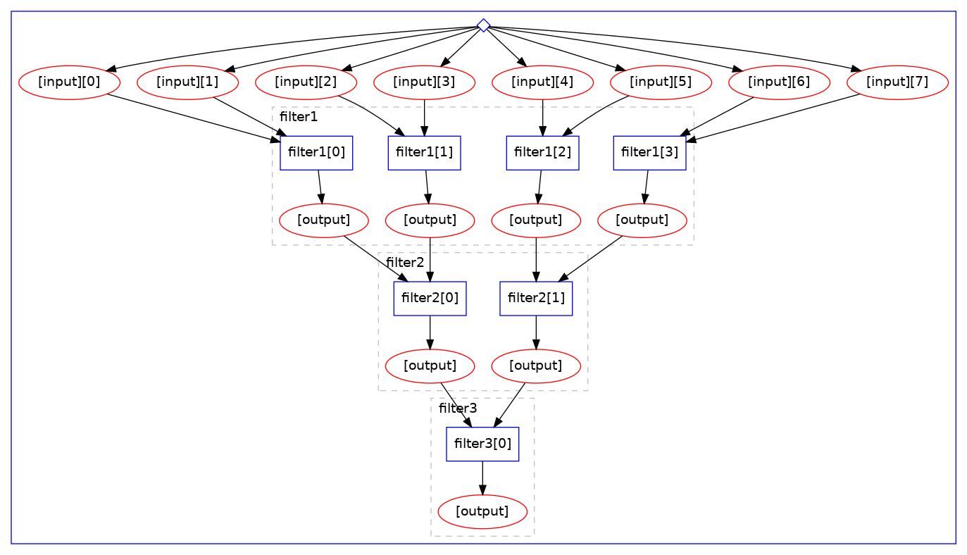
Note how the “scatter” operation is automatically happening over the given “input” array with the
wanted batch size, processing files two by two irrespective of the number of input files. Note
also the automatic “cascading” of computations.
Snakemake has several concepts how to parametrise calculations. One can start by using rule wildcards. For example, if we would like to process five data samples concurrently, you can specify rules like:
samples = ["1","2","3","4","5"]

rule scatter:
    input:
        "myinputs{n}.txt"
    output:
        "myresults{n}.txt"
    shell:
      ...

rule gather:
    input:
        expand("myresults{n}.txt", n=samples)
    output:
        "sum.txt"
    shell:
        ...
Here Snakemake will start five independent jobs to “scatter” computations over data, yielding
partial myresults.txt files for each sample, and then aggregates them as necessary in the “gather”
rule.
In the next episode we shall see how the scatter-gather paradigm can be used to speed up the HiggsToTauTau sequential workflow that we developed in the previous episode.
Key Points
Computational analysis is a graph of inter-dependent steps
Fully declare inputs and outputs for each step
Use dependencies between workflow steps to allow running jobs in parallel
Use scatter/gather paradigm to parallelise parametrised computations