Introduction

Overview

Teaching: 10 min
Exercises: 1 min

Questions

• What makes research data analyses reproducible?

• Is preserving code, data, and containers enough?

Objectives

• Understand principles behind computational reproducibility

• Understand the concept of serial and parallel computational workflow graphs

Computational reproducibility

A reproducibility quote

An article about computational science in a scientific publication is not the scholarship itself, it is merely advertising of the scholarship. The actual scholarship is the complete software development environment and the complete set of instructions which generated the figures.

– Jonathan B. Buckheit and David L. Donoho, “WaveLab and Reproducible Research”, source

Computational reproducibility has many definitions. The terms such as reproducibility, replicability, and repeatability have often different meaning in different scientific disciplines.

One possible point of view on the computational reproducibility is provided by The Turing Way: source

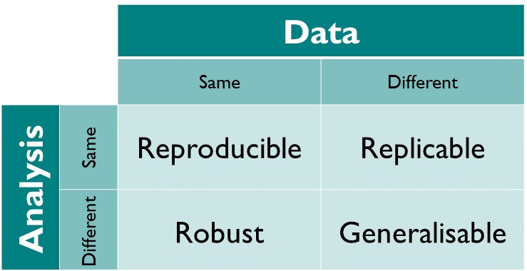
In other words, “same data + same analysis = reproducible results” (perhaps run on a different underlying computing architecture such as from Intel to ARM processors).

The more interesting use case is “reusable analyses”, i.e. testing the same theory on new data, or altering the theory and reinterpreting old data.

Another possible point of view on the computational reproducibility is provided by the PRIMAD model: source

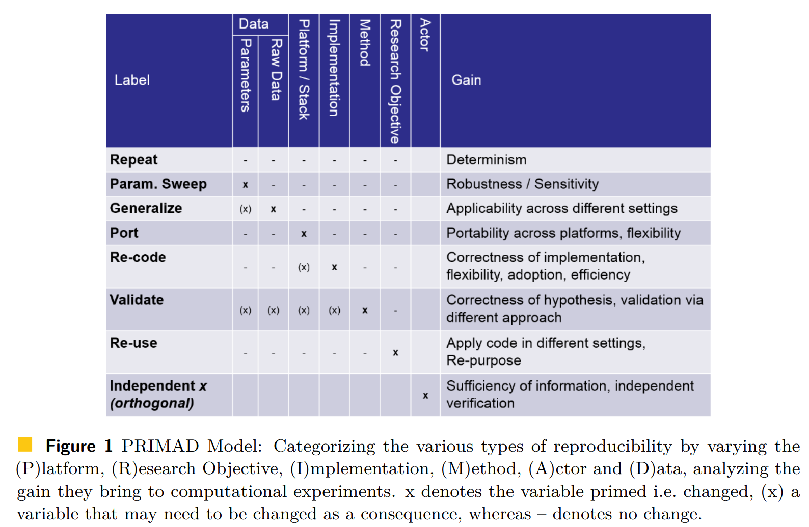
An analysis is reproducible, repeatable, reusable, robust if one can “wiggle” various parameters entering the process. For example, change platform (from Intel to ARM processors); is it portable? Or change the actor performing the analysis (from Alice to Bob); is it independent of the analyst?

The real life shows it often is not.

Example: Monya Baker published in Nature 533 (2016) 452-454 the results from surveying 1500 scientists: source

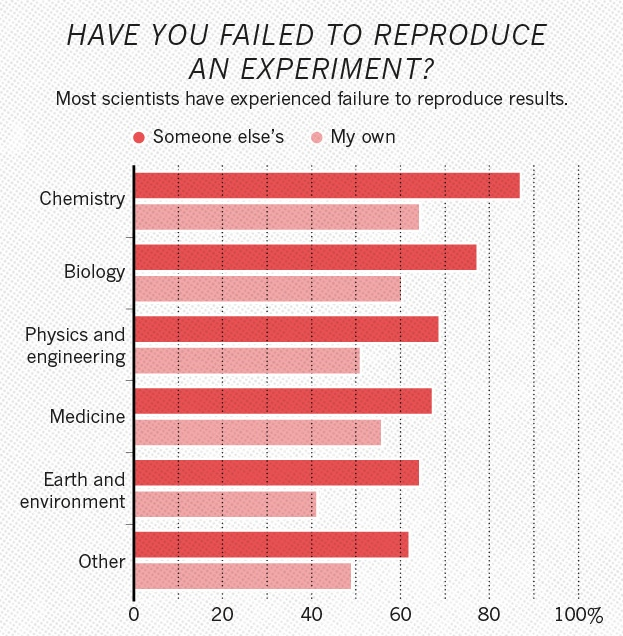
Half of researchers cannot reproduce even their own results. And physics is not doing visibly better than the other scientific disciplines.

Slow uptake of best practices

Many guidelines with “best practices” for computational reproducibility have been published. For example, “Ten Simple Rules for Reproducible Computational Research” by Geir Kjetil Sandve, Anton Nekrutenko, James Taylor, Eivind Hovig (2013) DOI:10.1371/journal.pcbi.1003285:

1. For every result, keep track of how it was produced
2. Avoid manual data manipulation steps
3. Archive the exact versions of all external programs used
4. Version control all custom scripts
5. Record all intermediate results, when possible in standardized formats
6. For analyses that include randomness, note underlying random seeds
7. Always store raw data behind plots
8. Generate hierarchical analysis output, allowing layers of increasing detail to be inspected
9. Connect textual statements to underlying results
10. Provide public access to scripts, runs, and results

Yet the uptake of good practices in real life has been slow. There are several reasons, including:

• sociological: publish-or-perish culture in scientific careers; missing incentives to create robust preserved and reusable technology stack;
• technological: easy-to-use tools for “active analyses” that would facilitate their future reuse.

The change is being brought by a combination of top-down approaches (e.g. funding bodies asking for Data Management Plans) and bottom-up approaches (building tools integrating into daily research workflows).

A reproducibility quote

Your closest collaborator is you six monhts ago… and your younger self does not reply to emails.

Four questions

Four questions to aid assessing the robustness of analyses:

1. Where is your input data? Specify all input data and input parameters that the analysis uses.
2. Where is your analysis code? Specify the analysis code and the software frameworks that are being used to analyse the data.
3. Which computing environment do you use? Specify the operating system platform that is used to run the analysis.
4. What are the computational steps to achieve the results? Specify all the commands and GUI clicks necessary to arrive at the final results.

The input data for statistical analyses, such as CMS MiniAOD, is produced centrally and the locations are well understood.

The analysis code and the containerised computational environments were covered in the previous two days of this workshop:

• HSF training on CI/CD
• HSF training on Docker

Exercise

Are containers enough to capture your runtime environment? What else might be necessary in your typical physics analysis scenarios?

Solution

Any external resources, such as condition database calls, must also be thought about. Will the external database that you use still be there and answering queries in the future?

Computational steps

Today’s lesson will focus mostly on the fourth question, i.e. the preservation of running computational steps.

The use of interactive and graphical interfaces is not recommended, since one cannot easily capture and reproduce user clicks.

The use of custom helper scripts (e.g. run.sh shell scripts), or custom orchestration scripts (e.g. Python glue code) running the analysis is much better.

However, porting glue code to new usage scenarios (for example to scale up to a new computer centre cluster) may be tedious technical word that would be better spent doing physics instead.

Hence the birth of declarative workflow systems that express the computational steps more abstractly.

Example of a serial computational workflow graph typical for ATLAS RECAST analyses:

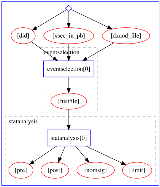
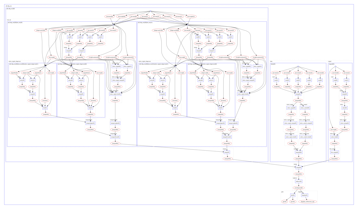
Example of a parallel computational workflow graph typical for Beyond Standard Model searches:

Many different computational data analysis workflow systems exist. Some are preferred to others because of the features they bring that others do not have, so there are fit-for-use and fit-for-purpose considerations. Some are preferred due to cultural differences in research teams or due to individual preferences.

In experimental particle physics, several such workflow systems are being used, for example Snakemake in LHCb or Yadage in ATLAS.

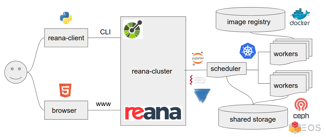
REANA

We shall use the REANA reproducible analysis platform to explore computational workflows in this lesson. REANA supports:

• multiple workflow systems (CWL, Serial, Snakemake, Yadage)
• multiple compute backends (Kubernetes, HTCondor, Slurm)

Analysis preservation ab initio

Preserving analysis code and processes after the publication is often coming too late. The key information and knowledge how to arrive at the results may get lost during the lengthy analysis process.

Hence the idea of making research reproducible from the start, in other words making research “preproducible”, to make the analysis preservation easy.

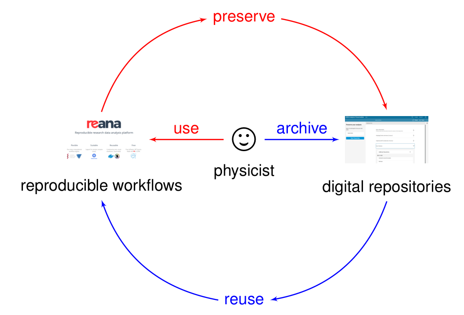
Preserve first and think about reusability later is the “blue pill” way.

Make analysis preproducible ab initio to facilitate its future preservation is the “red pill” way.

Key Points

• Workflow is the new data.

• Data + Code + Environment + Workflow = Reproducible Analyses

• Before reproducibility comes preproducibility