Introduction: Python background
Overview
Teaching: 20 min
Exercises: 5 minQuestions
How much Python do we need to know?
What is “array-oriented” or “columnar” processing?
What is a “software ecosystem”?
Objectives
Get the background context to get started with the Uproot lessons.
How much Python do we need to know?
Basic Python
Most students start this module after a Python introduction or are already familiar with the basics of Python. For instance, you should be comfortable with the Python essentials such as assigning variables,
x = 5
if-statements,
if x < 5:
    print("small")
else:
    print("big")
and loops.
for i in range(x):
    print(i)
Your data analysis will likely be full of statements like these, though the kinds of operations we’ll be focusing on in this module have a form more like
import compiled_library

compiled_library.do_computationally_expensive_thing(big_array)
The trick is for the Python-side code to be expressive enough and the compiled code to be general enough that you don’t need a new compiled_library for each thing you want to do. The libraries presented in this module are designed with interfaces that let you express what you want to do in Python and have it run in compiled code.
Dict-like and array-like interfaces
The two most important data types for these interfaces are dicts
some_dict = {"word": 1, "another word": 2, "some other word": 3}
some_dict["some other word"]
for key in some_dict:
    print(key, some_dict[key])
and arrays
import numpy as np

some_array = np.array([0.0, 1.1, 2.2, 3.3, 4.4, 5.5, 6.6, 7.7, 8.8, 9.9])
some_array[4]
for x in some_array:
    print(x)
Although these data types are important, what’s more important is the interfaces to these types. They both represent functions from keys to values:
- dicts (usually) map from strings to Python objects,
- arrays (always) map from non-negative integers to numerical values.
Most of the types we will see in this module also map strings or integers to data, and they use the same syntax as dicts and arrays. If you’re familiar with the dict and array interfaces, you usually won’t have to look up documentation on dict-like and array-like types unless you’re trying to do something special.
Review of the dict interface
For dicts, the things that can go in square brackets (its “domain,” as a function) are its keys.
some_dict = {"word": 1, "another word": 2, "some other word": 3}
some_dict.keys()
Nothing other than these keys can be used in square brackets
some_dict["something I made up"]
unless it has been added to the dict.
some_dict["something I made up"] = 123
some_dict["something I made up"]
The things that can come out of a dict (its “range,” as a function) are its values.
some_dict.values()
You can get keys and values as 2-tuples by asking for its items.
some_dict.items()

for key, value in some_dict.items():
    print(key, value)
Review of the array interface
For arrays, the things that can go in square brackets (its “domain,” as a function) are integers from zero up to but not including its length.
import numpy as np

some_array = np.array([0.0, 1.1, 2.2, 3.3, 4.4, 5.5, 6.6, 7.7, 8.8, 9.9])
some_array[0]  # okay
some_array[1]  # okay
some_array[9]  # okay
some_array[10]  # not okay
You can get the length of an array (and the number of keys in a dict) with len:
len(some_array)
It’s important to remember that index 0 corresponds to the first item in the array, 1 to the second, and so on, which is why len(some_array) is not a valid index.
Negative indexes are allowed, but they count from the end of the list to the beginning. For instance,
some_array[-1]
returns the last item. Quick quiz: which negative value returns the first item, equivalent to 0?
Arrays can also be “sliced” by putting a colon (:) between the starting and stopping index.
some_array[2:7]
Quick quiz: why is 7.7 not included in the output?
The above is common to all Python sequences. Arrays, however, can be multidimensional and this allows for more kinds of slicing.
array3d = np.arange(2 * 3 * 5).reshape(2, 3, 5)
Separating two slices in the square brackets with a comma
array3d[:, 1:, 1:]
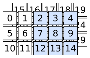
selects the following:
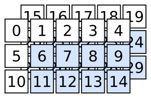
Quick quiz: how do you select the following?
Filtering with booleans and integers: “cuts”
In addition to integers and slices, arrays can be included in the square brackets.
An array of booleans with the same length as the sliced array selects all items that line up with True.
some_array = np.array([0.0, 1.1, 2.2, 3.3, 4.4, 5.5, 6.6, 7.7, 8.8, 9.9])
boolean_array = np.array(
    [True, True, True, True, True, False, True, False, True, False]
)

some_array[boolean_array]
An array of integers selects items by index.
some_array = np.array([0.0, 1.1, 2.2, 3.3, 4.4, 5.5, 6.6, 7.7, 8.8, 9.9])
integer_array = np.array([0, 1, 2, 3, 4, 6, 8])

some_array[integer_array]
Integer-slicing is more general than boolean-slicing because an array of integers can also change the order of the data and repeat items.
some_array[np.array([4, 2, 2, 2, 9, 8, 3])]
Both come up in natural contexts. Boolean arrays often come from performing a calculation on all elements of an array that returns boolean values.
even_valued_items = some_array * 10 % 2 == 0

some_array[even_valued_items]
This is how we’ll be computing and applying cuts: expressions like
good_muon_cut = (muons.pt > 10) & (abs(muons.eta) < 2.4)

good_muons = muons[good_muon_cut]
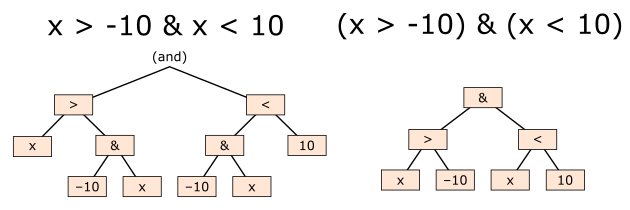
Logical operators: &, |, ~, and parentheses
If you’re coming from C++, you might expect “and,” “or,” “not” to be &&, ||, !.
If you’re coming from non-array Python, you might expect them to be and, or, not.
In array expressions (unfortunately!), we have to use Python’s bitwise operators, &, |, ~, and ensure that comparisons are surrounded in parentheses. Python’s and, or, not are not applied across arrays and bitwise operators have a surprising operator-precedence.
x = 0

x > -10 & x < 10  # probably not what you expect!

(x > -10) & (x < 10)
What is “array-oriented” or “columnar” processing?
Expressions like
even_valued_items = some_array * 10 % 2 == 0
perform the *, %, and == operations on every item of some_array and return arrays. Without NumPy, the above would have to be written as
even_valued_items = []

for x in some_array:
    even_valued_items.append(x * 10 % 2 == 0)
This is more cumbersome when you want to apply a mathematical formula to every item of a collection, but it is also considerably slower. Every step in a Python for loop performs sanity checks that are unnecessary for numerical values with uniform type, checks that would happen at compile-time in a compiled library. NumPy is a compiled library; its *, %, and == operators, as well as many other functions, are performed in fast, compiled loops.
This is how we get expressiveness and speed. Languages with operators that apply array at a time, rather than one scalar value at a time, are called “array-oriented” or “columnar” (referring to, for instance, Pandas DataFrame columns).
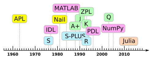
Quite a few interactive, data-analysis languages are array-oriented, deriving from the original APL. “Array-oriented” is a programming paradigm in the same sense as “functional” or “object-oriented.”
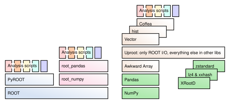
What is a “software ecosystem”?
Some programming environments, like Mathematica, Emacs, and ROOT, attempt to provide you with everything you need in one package. There’s only one thing to install and components within the framework should work well together because they were developed together. However, it can be hard to use the framework with other, unrelated software packages.
Ecosystems, like UNIX, iOS App Store, and Python, consist of many small software packages that each do one thing and know how to communicate with other packages through conventions and protocols. There’s usually a centralized installation mechanism, and it is the user’s (your) responsibility to piece together what you need. However, the set of possibilities is open-ended and grows as needs develop.
In mainstream Python, this means that
- NumPy only deals with arrays,
- Pandas only deals with tables,
- Matplotlib only plots,
- Jupyter only provides a notebook interface,
- Scikit-Learn only does machine learning,
- h5py only interfaces with HDF5 files,
- etc.
Python packages for high-energy physics are being developed with a similar model:
- Uproot only reads and writes ROOT files,
- Awkward Array only deals with arrays of irregular types,
- hist only deals with histograms,
- iminuit only optimizes,
- zfit only fits,
- Particle only provides PDG-style data,
- etc.
To make things easier to find, they’re cataloged under a common name at scikit-hep.org.

Key Points
Be familiar with the syntax of Python dicts, NumPy arrays, slicing rules, and bitwise logic operators.
Large-scale computations in Python tend to be performed one array at a time, rather than one scalar operation at a time.
You, as a user, will likely be gluing together many packages in each data analysis.
Basic file I/O with Uproot
Overview
Teaching: 25 min
Exercises: 0 minQuestions
How can I find my data in a ROOT file?
How can I plot it?
How can I write new data to a ROOT file?
Objectives
Learn how to navigate through a ROOT file.
Learn how to send ROOT data to the libraries that can act on them.
Learn how to write histograms and TTrees to files.
What is Uproot?
Uproot is a Python package that reads and writes ROOT files and is only concerned with reading and writing (no analysis, no plotting, etc.). It interacts with NumPy, Awkward Array, and Pandas for computations, boost-histogram/hist for histogram manipulation and plotting, Vector for Lorentz vector functions and transformations, Coffea for scale-up, etc.
Uproot is implemented using only Python and Python libraries. It doesn’t have a compiled part or require a specific version of ROOT. (This means that if you do use ROOT for something other than I/O, your choice of ROOT version is not constrained by I/O.)
As a consequence of being an independent implementation of ROOT I/O, Uproot might not be able to read/write certain data types. Which data types are not implemented is a moving target, as new ones are always being added. A good approach for reading data is to just try it and see if Uproot complains. For writing, see the lists of supported types in the Uproot documentation (blue boxes in the text).
Reading data from a file
Opening the file
To open a file for reading, pass the name of the file to uproot.open. In scripts, it is good practice to use Python’s with statement to close the file when you’re done, but if you’re working interactively, you can use a direct assignment.
import skhep_testdata

filename = skhep_testdata.data_path(
    "uproot-Event.root"
)  # downloads this test file and gets a local path to it

import uproot

file = uproot.open(filename)
To access a remote file via HTTP or XRootD, use a "http://...", "https://...", or "root://..." URL. If the Python interface to XRootD is not installed, the error message will explain how to install it.
Listing contents
This “file” object actually represents a directory, and the named objects in that directory are accessible with a dict-like interface. Thus, keys, values, and items return the key names and/or read the data. If you want to just list the objects without reading, use keys. (This is like ROOT’s ls(), except that you get a Python list.)
file.keys()
Often, you want to know the type of each object as well, so uproot.ReadOnlyDirectory objects also have a classnames method, which returns a dict of object names to class names (without reading them).
file.classnames()
Reading a histogram
If you’re familiar with ROOT, TH1F would be recognizable as histograms and TTree would be recognizable as a dataset. To read one of the histograms, put its name in square brackets:
h = file["hstat"]
h
Uproot doesn’t do any plotting or histogram manipulation, so the most useful methods of h begin with “to”: to_boost (boost-histogram), to_hist (hist), to_numpy (NumPy’s 2-tuple of contents and edges), to_pyroot (PyROOT), etc.
h.to_hist().plot()
Uproot histograms also satisfy the UHI plotting protocol, so they have methods like values (bin contents), variances (errors squared), and axes.
h.values()
h.variances()
list(h.axes[0])  # "x", "y", "z" or 0, 1, 2
Reading a TTree
A TTree represents a potentially large dataset. Getting it from the uproot.ReadOnlyDirectory only returns its TBranch names and types. The show method is a convenient way to list its contents:
t = file["T"]
t.show()
Be aware that you can get the same information from keys (an uproot.TTree is dict-like), typename, and interpretation.
t.keys()
t["event/fNtrack"]
t["event/fNtrack"].typename
t["event/fNtrack"].interpretation
(If an uproot.TBranch has no interpretation, it can’t be read by Uproot.)
The most direct way to read data from an uproot.TBranch is by calling its array method.
t["event/fNtrack"].array()
We’ll consider other methods in the next lesson.
Reading a… what is that?
This file also contains an instance of type TProcessID. These aren’t typically useful in data analysis, but Uproot manages to read it anyway because it follows certain conventions (it has “class streamers”). It’s presented as a generic object with an all_members property for its data members (through all superclasses).
file["ProcessID0"]
file["ProcessID0"].all_members
Here’s a more useful example of that: a supernova search with the IceCube experiment has custom classes for its data, which Uproot reads and represents as objects with all_members.
icecube = uproot.open(skhep_testdata.data_path("uproot-issue283.root"))
icecube.classnames()

icecube["config/detector"].all_members
icecube["config/detector"].all_members["ChannelIDMap"]
Writing data to a file
Uproot’s ability to write data is more limited than its ability to read data, but some useful cases are possible.
Opening files for writing
First of all, a file must be opened for writing, either by creating a completely new file or updating an existing one.
output1 = uproot.recreate("completely-new-file.root")
output2 = uproot.update("existing-file.root")
(Uproot cannot write over a network; output files must be local.)
Writing strings and histograms
These uproot.WritableDirectory objects have a dict-like interface: you can put data in them by assigning to square brackets.
output1["some_string"] = "This will be a TObjString."

output1["some_histogram"] = file["hstat"]

import numpy as np

output1["nested_directory/another_histogram"] = np.histogram(
    np.random.normal(0, 1, 1000000)
)
In ROOT, the name of an object is a property of the object, but in Uproot, it’s a key in the TDirectory that holds the object, so that’s why the name is on the left-hand side of the assignment, in square brackets. Only the data types listed in the blue box in the documentation are supported: mostly just histograms.
Writing TTrees
TTrees are potentially large and might not fit in memory. Generally, you’ll need to write them in batches.
One way to do this is to assign the first batch and extend it with subsequent batches:
import numpy as np

output1["tree1"] = {
    "x": np.random.randint(0, 10, 1000000),
    "y": np.random.normal(0, 1, 1000000),
}
output1["tree1"].extend(
    {"x": np.random.randint(0, 10, 1000000), "y": np.random.normal(0, 1, 1000000)}
)
output1["tree1"].extend(
    {"x": np.random.randint(0, 10, 1000000), "y": np.random.normal(0, 1, 1000000)}
)
another is to create an empty TTree with uproot.WritableDirectory.mktree, so that every write is an extension.
output1.mktree("tree2", {"x": np.int32, "y": np.float64})
output1["tree2"].extend(
    {"x": np.random.randint(0, 10, 1000000), "y": np.random.normal(0, 1, 1000000)}
)
output1["tree2"].extend(
    {"x": np.random.randint(0, 10, 1000000), "y": np.random.normal(0, 1, 1000000)}
)
output1["tree2"].extend(
    {"x": np.random.randint(0, 10, 1000000), "y": np.random.normal(0, 1, 1000000)}
)
Performance tips are given in the next lesson, but in general, it pays to write few large batches, rather than many small batches.
The only data types that can be assigned or passed to extend are listed in the blue box in this documentation. This includes jagged arrays (described in the lesson after next), but not more complex types.
Reading and writing RNTuples
TTree has been the default format to store large datasets in ROOT files for decades. However, it has slowly become outdated and are not optimized for modern systems. This is where the RNTuple format comes in. It is a modern serialization format that is designed with modern systems in mind and is planned to replace TTree in the coming years. Version 1.0.0.0 is out and will be supported “forever”.
RNTuples are much simpler than TTrees by design, and this time there is an official specification, which makes it much easier for third-party I/O packages like Uproot to support. Uproot already supports reading the full RNTuple specification, meaning that you can read any RNTuple you find in the wild. It also supports writing a large part of the specification, and intends to support as much as it makes sense for data analysis.
To ease the transition into RNTuples, we are designing the interface to match the one for TTrees as closely as possible. Let’s look at a simple example for reading and writing RNTuples.
Again, we’ll use a sample file from the
filename = skhep_testdata.data_path("ntpl001_staff_rntuple_v1-0-0-0.root")

file = uproot.open(filename)
This time, if we print the class names, we see that there is an RNTuple instead of a TTree.
file.classnames()
Then to read the data from the RNTuple works in an analogous way.
rntuple = file["Staff"]
data = rntuple.arrays()
Writing again works in a very similar way to TTrees. However, since TTrees are still the default format used in more places, writing something like file[key] = data will default to writing the data as a TTree. When we want to write an RNTuple, we need to specifically tell Uproot that we want to do so. For now, we need to use an Awkward Array (which will be covered in a later lesson) to specify the data, but the interface will be extended to match TTrees.
import awkward as ak

data = ak.Array({"my_int_data": [1, 2, 3], "my_float_data": [1.0, 2.0, 3.0]})
more_data = ak.Array({"my_int_data": [4, 5, 6], "my_float_data": [4.0, 5.0, 6.0]})

output3 = uproot.recreate("new-file-with-rntuple.root")

rntuple = output3.mkrntuple("my_rntuple", data)
rntuple.extend(more_data)
For the rest of the tutorial we will stick to using TTrees since this is still the main data format that you’ll encounter for now.
Key Points
Uproot TDirectories and TTrees have a dict-like interface.
Uproot reading methods are primarily intended to get data into a more specialized library.
Uproot writing is more limited, but it can write histograms and TTrees.
TTree details
Overview
Teaching: 25 min
Exercises: 0 minQuestions
What are TBranches and TBaskets?
How can I read multiple TBranches at once?
How can I get ROOT data into NumPy or Pandas?
Objectives
Learn how to read over TTrees efficiently, including common pitfalls.
Learn how to turn interactive tinkering into a scaled-up job.
Learn how to send data directly into NumPy or Pandas.
ROOT file structure and terminology
A ROOT file (ROOT TFile, uproot.ReadOnlyFile) is like a little filesystem containing nested directories (ROOT TDirectory, uproot.ReadOnlyDirectory). In Uproot, nested directories are presented as nested dicts.
Any class instance (ROOT TObject, uproot.Model) can be stored in a directory, including types such as histograms (e.g. ROOT TH1, uproot.behaviors.TH1.TH1).
One of these classes, TTree (ROOT TTree, uproot.TTree), is a gateway to large datasets. A TTree is roughly like a Pandas DataFrame in that it represents a table of data. The columns are called TBranches (ROOT TBranch, uproot.TBranch), which can be nested (unlike Pandas), and the data can have any C++ type (unlike Pandas, which can store any Python type).
A TTree is often too large to fit in memory, and sometimes (rarely) even a single TBranch is too large to fit in memory. Each TBranch is therefore broken down into TBaskets (ROOT TBasket, uproot.models.TBasket.Model_TBasket), which are “batches” of data. (These are the same batches that each call to extend writes in the previous lesson.) TBaskets are the smallest unit that can be read from a TTree: if you want to read the first entry, you have to read the first TBasket.
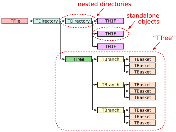
As a data analyst, you’ll likely be concerned with TTrees and TBranches first-hand, but only TBaskets when efficiency issues come up. Files with large TBaskets might require a lot of memory to read; files with small TBaskets will be slower to read (in ROOT also, but especially in Uproot). Megabyte-sized TBaskets are usually ideal.
Examples with a large TTree
This file is 2.1 GB, hosted by CERN’s Open Data Portal.
import uproot

file = uproot.open(
    "root://eospublic.cern.ch//eos/opendata/cms/derived-data/AOD2NanoAODOutreachTool/Run2012BC_DoubleMuParked_Muons.root"
)
file.classnames()
Why the
;74and;75?You may have been wondering about the numbers after the semicolons. These are ROOT “cycle numbers,” which allow objects with the same name to be distinguishable. They’re used when an object needs to be overwritten as it grows without losing the last valid copy of that object, so that a ROOT file can be read even if the writing process failed partway through.
In this case, the last version of this TTree was number 75, and number 74 is the second-to-last.
If you don’t specify cycle numbers, Uproot will pick the last for you, which is almost always what you want. (In other words, you can ignore them.)
Just asking for the uproot.TTree object and printing it out does not read the whole dataset.
tree = file["Events"]
tree.show()
Reading part of a TTree
In the last lesson, we learned that the most direct way to read one TBranch is to call uproot.TBranch.array.
tree["nMuon"].array()
However, it takes a long time because a lot of data have to be sent over the network.
To limit the amount of data read, set entry_start and entry_stop to the range you want. The entry_start is inclusive, entry_stop exclusive, and the first entry would be indexed by 0, just like slices in an array interface (first lesson). Uproot only reads as many TBaskets as are needed to provide these entries.
tree["nMuon"].array(entry_start=1_000, entry_stop=2_000)
These are the building blocks of a parallel data reader: each is responsible for a different slice. (See also uproot.TTree.num_entries_for and uproot.TTree.common_entry_offsets, which can be used to pick entry_start/entry_stop in optimal ways.)
Reading multiple TBranches at once
Suppose you know that you will need all of the muon TBranches. Asking for them in one request is more efficient than asking for each TBranch individually because the server can be working on reading the later TBaskets from disk while the earlier TBaskets are being sent over the network to you. Whereas a TBranch has an array method, the TTree has an arrays (plural) method for getting multiple arrays.
muons = tree.arrays(
    ["Muon_pt", "Muon_eta", "Muon_phi", "Muon_mass", "Muon_charge"], entry_stop=1_000
)
muons
Now all five of these TBranches are in the output, muons, which is an Awkward Array. An Awkward Array of multiple TBranches has a dict-like interface, so we can get each variable from it by
muons["Muon_pt"]
muons["Muon_eta"]
muons["Muon_phi"]  # etc.
Beware! It’s
tree.arraysthat actually reads the data!If you’re not careful with the uproot.TTree.arrays call, you could end up waiting a long time for data you don’t want or you could run out of memory. Reading everything with
everything = tree.arrays()and then picking out the arrays you want is usually not a good idea. At the very least, set an
entry_stop.
Selecting TBranches by name
Suppose you have many muon TBranches and you don’t want to list them all. The uproot.TTree.keys and uproot.TTree.arrays both take a filter_name argument that can select them in various ways (see documentation). In particular, it’s good to use the keys first, to know which branches match your filter, followed by arrays, to actually read them.
tree.keys(filter_name="Muon_*")

tree.arrays(filter_name="Muon_*", entry_stop=1_000)
(There are also filter_typename and filter_branch for more options.)
Scaling up, making a plot
The best way to figure out what you’re doing is to tinker with small datasets, and then scale them up. Here, we take 1000 events and compute dimuon masses.
muons = tree.arrays(entry_stop=1_000)
cut = muons["nMuon"] == 2

pt0 = muons["Muon_pt", cut, 0]
pt1 = muons["Muon_pt", cut, 1]
eta0 = muons["Muon_eta", cut, 0]
eta1 = muons["Muon_eta", cut, 1]
phi0 = muons["Muon_phi", cut, 0]
phi1 = muons["Muon_phi", cut, 1]

import numpy as np

mass = np.sqrt(2 * pt0 * pt1 * (np.cosh(eta0 - eta1) - np.cos(phi0 - phi1)))

import hist

masshist = hist.Hist(hist.axis.Regular(120, 0, 120, label="mass [GeV]"))
masshist.fill(mass)
masshist.plot()
That worked (there’s a Z peak). Now to do this over the whole file, we should be more careful about what we’re reading,
tree.keys(filter_name=["nMuon", "/Muon_(pt|eta|phi)/"])
and accumulate data gradually with uproot.TTree.iterate. This handles the entry_start/entry_stop in a loop.
masshist = hist.Hist(hist.axis.Regular(120, 0, 120, label="mass [GeV]"))

for muons in tree.iterate(filter_name=["nMuon", "/Muon_(pt|eta|phi)/"]):
    cut = muons["nMuon"] == 2
    pt0 = muons["Muon_pt", cut, 0]
    pt1 = muons["Muon_pt", cut, 1]
    eta0 = muons["Muon_eta", cut, 0]
    eta1 = muons["Muon_eta", cut, 1]
    phi0 = muons["Muon_phi", cut, 0]
    phi1 = muons["Muon_phi", cut, 1]
    mass = np.sqrt(2 * pt0 * pt1 * (np.cosh(eta0 - eta1) - np.cos(phi0 - phi1)))
    masshist.fill(mass)
    print(masshist.sum() / tree.num_entries)

masshist.plot()
Getting data into NumPy or Pandas
In all of the above examples, the array, arrays, and iterate methods return Awkward Arrays. The Awkward Array library is useful for exactly this kind of data (jagged arrays: more in the next lesson), but you might be working with libraries that only recognize NumPy arrays or Pandas DataFrames.
Use library="np" or library="pd" to get NumPy or Pandas, respectively.
tree["nMuon"].array(library="np", entry_stop=10_000)

tree.arrays(library="np", entry_stop=10_000)

tree.arrays(library="pd", entry_stop=10_000)
NumPy is great for non-jagged data like the "nMuon" branch, but it has to represent an unknown number of muons per event as an array of NumPy arrays (i.e. Python objects).
Pandas can be made to represent multiple particles per event by putting this structure in a pd.MultiIndex, but not when the DataFrame contains more than one particle type (e.g. muons and electrons). Use separate DataFrames for these cases. If it helps, note that there’s another route to DataFrames: by reading the data as an Awkward Array and calling ak.to_pandas on it. (Some methods use more memory than others, and I’ve found Pandas to be unusually memory-intensive.)
Or use Awkward Arrays (next lesson).
Key Points
ROOT files have a structure that enables partial reading. This is essential for large datasets.
Be aware of how much data you’re reading and when.
The Python + Jupyter + Uproot interface provides a gradual path from interactive tinkering to scaled-up workflows.
Jagged, ragged, Awkward Arrays
Overview
Teaching: 30 min
Exercises: 15 minQuestions
How do I cut particles, rather than events?
How do I compute quantities on combinations of particles?
Objectives
Learn how to slice and perform computations on irregularly shaped arrays.
Apply these skills to improve the dimuon mass spectrum.
What is Awkward Array?
The previous lesson included a tricky slice:
cut = muons["nMuon"] == 2

pt0 = muons["Muon_pt", cut, 0]
The three parts of muons["Muon_pt", cut, 0] slice
- selects the
"Muon_pt"field of all records in the array, - applies
cut, a boolean array, to select only events with two muons, - selects the first (
0) muon from each of those pairs. Similarly for the second (1) muons.
NumPy would not be able to perform such a slice, or even represent an array of variable-length lists without resorting to arrays of objects.
import numpy as np

# generates a ValueError
np.array([[0.0, 1.1, 2.2], [], [3.3, 4.4], [5.5], [6.6, 7.7, 8.8, 9.9]])
Awkward Array is intended to fill this gap:
import awkward as ak

ak.Array([[0.0, 1.1, 2.2], [], [3.3, 4.4], [5.5], [6.6, 7.7, 8.8, 9.9]])
Arrays like this are sometimes called “jagged arrays” and sometimes “ragged arrays.”
Slicing in Awkward Array
Basic slices are a generalization of NumPy’s—what NumPy would do if it had variable-length lists.
array = ak.Array([[0.0, 1.1, 2.2], [], [3.3, 4.4], [5.5], [6.6, 7.7, 8.8, 9.9]])
array.tolist()

array[2]
array[-1, 1]
array[2:, 0]
array[2:, 1:]
array[:, 0]
Quick quiz: why does the last one raise an error?
Boolean and integer slices work, too:
array[[True, False, True, False, True]]

array[[2, 3, 3, 1]]
Like NumPy, boolean arrays for slices can be computed, and functions like ak.num are helpful for that.
ak.num(array)

ak.num(array) > 0

array[ak.num(array) > 0, 0]
array[ak.num(array) > 1, 1]
Now consider this (similar to an example from the first lesson):
cut = array * 10 % 2 == 0

array[cut]
This array, cut, is not just an array of booleans. It’s a jagged array of booleans. All of its nested lists fit into array’s nested lists, so it can deeply select numbers, rather than selecting lists.
Application: selecting particles, rather than events
Returning to the big TTree from the previous lesson,
import uproot

file = uproot.open(
    "root://eospublic.cern.ch//eos/opendata/cms/derived-data/AOD2NanoAODOutreachTool/Run2012BC_DoubleMuParked_Muons.root"
)
tree = file["Events"]

muon_pt = tree["Muon_pt"].array(entry_stop=10)
This jagged array of booleans selects all muons with at least 20 GeV:
particle_cut = muon_pt > 20

muon_pt[particle_cut]
and this non-jagged array of booleans (made with ak.any) selects all events that have a muon with at least 20 GeV:
event_cut = ak.any(muon_pt > 20, axis=1)

muon_pt[event_cut]
Quick quiz: construct exactly the same event_cut using ak.max.
Quick quiz: apply both cuts; that is, select muons with over 20 GeV from events that have them.
Hint: you’ll want to make a
cleaned = muon_pt[particle_cut]
intermediary and you can’t use the variable event_cut, as-is.
Hint: the final result should be a jagged array, just like muon_pt, but with fewer lists and fewer items in those lists.
Solution (no peeking!)
cleaned = muon_pt[particle_cut]
final_result = cleaned[event_cut]
final_result.tolist()
[[32.911224365234375, 23.72175407409668],
[57.6067008972168, 53.04507827758789],
[23.906352996826172]]
Combinatorics in Awkward Array
Variable-length lists present more problems than just slicing and computing formulas array-at-a-time. Often, we want to combine particles in all possible pairs (within each event) to look for decay chains.
Pairs from two arrays, pairs from a single array
Awkward Array has functions that generate these combinations. For instance, ak.cartesian takes a Cartesian product per event (when axis=1, the default).
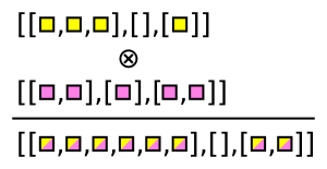
numbers = ak.Array([[1, 2, 3], [], [5, 7], [11]])
letters = ak.Array([["a", "b"], ["c"], ["d"], ["e", "f"]])

pairs = ak.cartesian((numbers, letters))
These pairs are 2-tuples, which are like records in how they’re sliced out of an array: using strings.
pairs["0"]
pairs["1"]
There’s also ak.unzip, which extracts every field into a separate array (opposite of ak.zip).
lefts, rights = ak.unzip(pairs)
lefts
rights
Note that these lefts and rights are not the original numbers and letters: they have been duplicated and have the same shape.
The Cartesian product is equivalent to this C++ for loop over two collections:
for (int i = 0; i < numbers.size(); i++) {
  for (int j = 0; j < letters.size(); j++) {
    // compute formula with numbers[i] and letters[j]
  }
}
Sometimes, though, we want to find all pairs within a single collection, without repetition. That would be equivalent to this C++ for loop:
for (int i = 0; i < numbers.size(); i++) {
  for (int j = i + 1; i < numbers.size(); j++) {
    // compute formula with numbers[i] and numbers[j]
  }
}
The Awkward function for this case is ak.combinations.
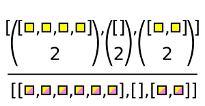
pairs = ak.combinations(numbers, 2)
pairs

lefts, rights = ak.unzip(pairs)

lefts * rights  # they line up, so we can compute formulas
Application to dimuons
The dimuon search in the previous lesson was a little naive in that we required exactly two muons to exist in every event and only computed the mass of that combination. If a third muon were present because it’s a complex electroweak decay or because something was mismeasured, we would be blind to the other two muons. They might be real dimuons.
A better procedure would be to look for all pairs of muons in an event and apply some criteria for selecting them.
In this example, we’ll ak.zip the muon variables together into records.
import uproot
import awkward as ak

file = uproot.open(
    "root://eospublic.cern.ch//eos/opendata/cms/derived-data/AOD2NanoAODOutreachTool/Run2012BC_DoubleMuParked_Muons.root"
)
tree = file["Events"]

arrays = tree.arrays(filter_name="/Muon_(pt|eta|phi|charge)/", entry_stop=10000)

muons = ak.zip(
    {
        "pt": arrays["Muon_pt"],
        "eta": arrays["Muon_eta"],
        "phi": arrays["Muon_phi"],
        "charge": arrays["Muon_charge"],
    }
)

arrays.type
muons.type
The difference between arrays and muons is that arrays contains separate lists of "Muon_pt", "Muon_eta", "Muon_phi", "Muon_charge", while muons contains lists of records with "pt", "eta", "phi", "charge" fields.
Now we can compute pairs of muon objects
pairs = ak.combinations(muons, 2)

pairs.type
and separate them into arrays of the first muon and the second muon in each pair.
mu1, mu2 = ak.unzip(pairs)
Quick quiz: how would you ensure that all lists of records in mu1 and mu2 have the same lengths? Hint: see ak.num and ak.all.
Since they do have the same lengths, we can use them in a formula.
import numpy as np

mass = np.sqrt(
    2 * mu1.pt * mu2.pt * (np.cosh(mu1.eta - mu2.eta) - np.cos(mu1.phi - mu2.phi))
)
Quick quiz: how many masses do we have in each event? How does this compare with muons, mu1, and mu2?
Plotting the jagged array
Since this mass is a jagged array, it can’t be directly histogrammed. Histograms take a set of numbers as inputs, but this array contains lists.
Supposing you just want to plot the numbers from the lists, you can use ak.flatten to flatten one level of list or ak.ravel to flatten all levels.
import hist

hist.Hist(hist.axis.Regular(120, 0, 120, label="mass [GeV]")).fill(
    ak.ravel(mass)
).plot()
Alternatively, suppose you want to plot the maximum mass-candidate in each event, biasing it toward Z bosons? ak.max is a different function that picks one element from each list, when used with axis=1.
ak.max(mass, axis=1)
Some values are None because there is no maximum of an empty list. ak.flatten/ak.ravel remove missing values (None) as well as squashing lists,
ak.flatten(ak.max(mass, axis=1), axis=0)
but so does removing the empty lists in the first place.
ak.max(mass[ak.num(mass) > 0], axis=1)
Exercise: select pairs of muons with opposite charges
This is neither an event-level cut nor a particle-level cut, it is a cut on particle pairs.
Solution (no peeking!)
The
mu1andmu2variables are the left and right halves of muon pairs. Therefore,cut = (mu1.charge != mu2.charge)has the right multiplicity to be applied to the
massarray.hist.Hist(hist.axis.Regular(120, 0, 120, label="mass [GeV]")).fill( ak.ravel(mass[cut]) ).plot()plots the cleaned muon pairs.
Exercise (harder): plot the one mass candidate per event that is strictly closest to the Z mass
Instead of just taking the maximum mass in each event, find the one with the minimum difference between computed mass and
zmass = 91.Hint: use ak.argmin with
keepdims=True.Anticipating one of the future lessons, you could get a more accurate mass by asking the Particle library:
import particle, hepunits

zmass = particle.Particle.findall("Z0")[0].mass / hepunits.GeV
Solution (no peeking!)
Instead of maximizing
mass, we want to minimizeabs(mass - zmass)and apply that choice tomass. ak.argmin returns the index position of this minimum difference, which we can then apply to the originalmass. However, withoutkeepdims=True, ak.argmin removes the dimension we would need for this array to have the same nested shape asmass. Therefore, wekeepdims=Trueand then use ak.ravel to get rid of missing values and flatten lists.The last step would require two applications of ak.flatten: one for squashing lists at the first level and another for removing
Noneat the second level.which = ak.argmin(abs(mass - zmass), axis=1, keepdims=True) hist.Hist(hist.axis.Regular(120, 0, 120, label="mass [GeV]")).fill( ak.ravel(mass[which]) ).plot()
Key Points
NumPy (and almost all array libraries) is only for rectilinear collections of numbers: arrays, tables, and tensors.
Awkward Array extends NumPy’s slicing and array-manipulation to jagged arrays and more general data types (such as nested records).
These extensions are useful for physics.
There’s usually more than one way to get what you want.
Histogram manipulations and fitting
Overview
Teaching: 15 min
Exercises: 0 minQuestions
How do I fill histograms?
How do I project/slice/rebin pre-filled histograms?
How do I fit histograms?
Objectives
Learn how high-energy physics histogramming differs from mainstream Python.
Learn about boost-histogram and hist, with their array-like slicing syntax.
See some examples of fitting histograms, using different packages.
Histogram libraries
Mainstream Python has libraries for filling histograms.
NumPy
NumPy, for instance, has an np.histogram function.
import skhep_testdata, uproot

tree = uproot.open(skhep_testdata.data_path("uproot-Zmumu.root"))["events"]

import numpy as np

np.histogram(tree["M"].array())
Because of NumPy’s prominence, this 2-tuple of arrays (bin contents and edges) is a widely recognized histogram format, though it lacks many of the features high-energy physicists expect (under/overflow, axis labels, uncertainties, etc.).
Matplotlib
Matplotlib also has a plt.hist function.
import matplotlib.pyplot as plt

plt.hist(tree["M"].array())
In addition to the same bin contents and edges as NumPy, Matplotlib includes a plottable graphic.
Boost-histogram and hist
The main feature that these functions lack (without some effort) is refillability. High-energy physicists usually want to fill histograms with more data than can fit in memory, which means setting bin intervals on an empty container and filling it in batches (sequentially or in parallel).
Boost-histogram is a library designed for that purpose. It is intended as an infrastructure component. You can explore its “low-level” functionality upon importing it:
import boost_histogram as bh
A more user-friendly layer (with plotting, for instance) is provided by a library called “hist.”
import hist

h = hist.Hist(hist.axis.Regular(120, 60, 120, name="mass"))

h.fill(tree["M"].array())

h.plot()
Universal Histogram Indexing (UHI)
There is an attempt within Scikit-HEP to standardize what array-like slices mean for a histogram. (See documentation.)
Naturally, integer slices should select a range of bins,
h[10:110].plot()
but often you want to select bins by coordinate value
# Explicit version
h[hist.loc(90) :].plot()

# Short version
h[90j:].plot()
or rebin by a factor,
# Explicit version
h[:: hist.rebin(2)].plot()

# Short version
h[::2j].plot()
or sum over a range.
# Explicit version
h[hist.loc(80) : hist.loc(100) : sum]

# Short version
h[90j:100j:sum]
Things get more interesting when a histogram has multiple dimensions.
import uproot
import hist
import awkward as ak

picodst = uproot.open(
    "https://pivarski-princeton.s3.amazonaws.com/pythia_ppZee_run17emb.picoDst.root:PicoDst"
)

vertexhist = hist.Hist(
    hist.axis.Regular(600, -1, 1, label="x"),
    hist.axis.Regular(600, -1, 1, label="y"),
    hist.axis.Regular(40, -200, 200, label="z"),
)

vertex_data = picodst.arrays(filter_name="*mPrimaryVertex[XYZ]")

vertexhist.fill(
    ak.flatten(vertex_data["Event.mPrimaryVertexX"]),
    ak.flatten(vertex_data["Event.mPrimaryVertexY"]),
    ak.flatten(vertex_data["Event.mPrimaryVertexZ"]),
)

vertexhist[:, :, sum].plot2d_full()
vertexhist[-0.25j:0.25j, -0.25j:0.25j, sum].plot2d_full()
vertexhist[sum, sum, :].plot()
vertexhist[-0.25j:0.25j:sum, -0.25j:0.25j:sum, :].plot()
A histogram object can have more dimensions than you can reasonably visualize—you can slice, rebin, and project it into something visual later.
Fitting histograms
By directly writing a loss function in Minuit:
import numpy as np
import iminuit.cost

norm = len(h.axes[0].widths) / (h.axes[0].edges[-1] - h.axes[0].edges[0]) / h.sum()


def f(x, background, mu, gamma):
    return (
        background
        + (1 - background) * gamma**2 / ((x - mu) ** 2 + gamma**2) / np.pi / gamma
    )


loss = iminuit.cost.LeastSquares(
    h.axes[0].centers, h.values() * norm, np.sqrt(h.variances()) * norm, f
)
loss.mask = h.variances() > 0

minimizer = iminuit.Minuit(loss, background=0, mu=91, gamma=4)

minimizer.migrad()
minimizer.hesse()

(h * norm).plot()
plt.plot(loss.x, f(loss.x, *minimizer.values))
Or through zfit, a Pythonic RooFit-like fitter:
import zfit

binned_data = zfit.data.BinnedData.from_hist(h)

binning = zfit.binned.RegularBinning(120, 60, 120, name="mass")
space = zfit.Space("mass", binning=binning)

background = zfit.Parameter("background", 0)
mu = zfit.Parameter("mu", 91)
gamma = zfit.Parameter("gamma", 4)
unbinned_model = zfit.pdf.SumPDF(
    [zfit.pdf.Uniform(60, 120, space), zfit.pdf.Cauchy(mu, gamma, space)], [background]
)

model = zfit.pdf.BinnedFromUnbinnedPDF(unbinned_model, space)
loss = zfit.loss.BinnedNLL(model, binned_data)

minimizer = zfit.minimize.Minuit()
result = minimizer.minimize(loss)

binned_data.to_hist().plot(density=1)
model.to_hist().plot(density=1)
Key Points
High-energy physicists approach histogramming in a different way from NumPy, Matplotlib, SciPy, etc.
Scikit-HEP tools make histogramming and fitting Pythonic.
Lorentz vectors, particle PDG IDs, jet-clustering, oh my!
Overview
Teaching: 15 min
Exercises: 0 minQuestions
How do I compute deltaR, mass, coordinate transformations, etc.?
How do I get masses, decay widths, and other particle properties?
What about jet-clustering and other specialized algorithms?
Objectives
Learn about the existence of some helpful Scikit-HEP packages.
Lorentz vectors
In keeping with the “many small packages” philosophy, 2D/3D/Lorentz vectors are handled by a package named Vector. This is where you can find calculations like deltaR and coordinate transformations.
import vector

one = vector.obj(px=1, py=0, pz=0)
two = vector.obj(px=0, py=1, pz=1)

one + two

one.deltaR(two)

one.to_rhophieta()
two.to_rhophieta()
To fit in with the rest of the ecosystem, Vector must be an array-oriented library. Arrays of 2D/3D/Lorentz vectors are processed in bulk.
MomentumNumpy2D, MomentumNumpy3D, MomentumNumpy4D are NumPy array subtypes: NumPy arrays can be cast to these types and get all the vector functions.
import skhep_testdata, uproot
import awkward as ak
import vector

tree = uproot.open(skhep_testdata.data_path("uproot-Zmumu.root"))["events"]

one = ak.to_numpy(tree.arrays(filter_name=["E1", "p[xyz]1"]))
two = ak.to_numpy(tree.arrays(filter_name=["E2", "p[xyz]2"]))

one.dtype.names = ("E", "px", "py", "pz")
two.dtype.names = ("E", "px", "py", "pz")

one = one.view(vector.MomentumNumpy4D)
two = two.view(vector.MomentumNumpy4D)

one + two

one.deltaR(two)

one.to_rhophieta()
two.to_rhophieta()
After vector.register_awkward() is called, "Momentum2D", "Momentum3D", "Momentum4D" are record names that Awkward Array will recognize to get all the vector functions.
vector.register_awkward()

tree = uproot.open(skhep_testdata.data_path("uproot-HZZ.root"))["events"]

array = tree.arrays(filter_name=["Muon_E", "Muon_P[xyz]"])

muons = ak.zip(
    {"px": array.Muon_Px, "py": array.Muon_Py, "pz": array.Muon_Pz, "E": array.Muon_E},
    with_name="Momentum4D",
)
mu1, mu2 = ak.unzip(ak.combinations(muons, 2))

mu1 + mu2

mu1.deltaR(mu2)

muons.to_rhophieta()
Particle properties and PDG identifiers
The Particle library provides all of the particle masses, decay widths and more from the PDG. It further contains a series of tools to programmatically query particle properties and use several identification schemes.
import particle
from hepunits import GeV

particle.Particle.findall("pi")

z_boson = particle.Particle.from_name("Z0")
z_boson.mass / GeV, z_boson.width / GeV

print(z_boson.describe())

particle.Particle.from_pdgid(111)

particle.Particle.findall(
    lambda p: p.pdgid.is_meson and p.pdgid.has_strange and p.pdgid.has_charm
)

print(particle.PDGID(211).info())

pdgid = particle.Corsika7ID(11).to_pdgid()
particle.Particle.from_pdgid(pdgid)
Jet clustering
In a high-energy pp collision, for instance, a spray of hadrons is produced which is clustered into `jets’ of particles and this method/process is called jet-clustering. The anti-kt jet clustering algorithm is one such algorithm used to combine particles/hadrons that are close to each other into jets.
Some people need to do jet-clustering at the analysis level. The fastjet package makes it possible to do that an (Awkward) array at a time.
import skhep_testdata, uproot
import awkward as ak
import particle
from hepunits import GeV
import vector

vector.register_awkward()

picodst = uproot.open(
    "https://pivarski-princeton.s3.amazonaws.com/pythia_ppZee_run17emb.picoDst.root:PicoDst"
)
px, py, pz = ak.unzip(
    picodst.arrays(filter_name=["Track/Track.mPMomentum[XYZ]"], entry_stop=100)
)

probable_mass = particle.Particle.from_name("pi+").mass / GeV

pseudojets = ak.zip(
    {"px": px, "py": py, "pz": pz, "mass": probable_mass}, with_name="Momentum4D"
)
good_pseudojets = pseudojets[pseudojets.pt > 0.1]

import fastjet

jetdef = fastjet.JetDefinition(fastjet.antikt_algorithm, 1.0)

clusterseq = fastjet.ClusterSequence(good_pseudojets, jetdef)
clusterseq.inclusive_jets()

ak.num(good_pseudojets), ak.num(clusterseq.inclusive_jets())
This fastjet package uses Vector to get coordinate transformations and all the Lorentz vector methods you’re accustomed to having in pseudo-jet objects. I used Particle to impute the mass of particles with only track-level information.
See how all the pieces accumulate?
Key Points
Instead of building vector methods into multiple packages, a standalone package provides just that.
The value of these small packages amplify when used together.
Tools for scaling up
Overview
Teaching: 10 min
Exercises: 0 minQuestions
How do I turn working code fragments into batch jobs?
Where can I look for more help?
Objectives
Learn where to go next.
Scaling up
The tools described in these lessons are intended to be used within a script that is scaled up for large datasets.
You could use any of them in an ordinary GRID job (or other batch processor).
However, the Coffea project (documentation) is building a distributed ecosystem that integrates Pythonic analysis with data analysis farms. This is too large of a subject to cover here, but check out the software and join the Coffea user meetings if you’re interested.
Scikit-HEP Resources
- scikit-hep.org
- Uproot GitHub, documentation
- Awkward Array GitHub, documentation
- boost-histogram GitHub, documentation
- hist GitHub, documentation
- Unified Histogram Interface GitHub, documentation
- mplhep GitHub, documentation
- iminuit GitHub, documentation
- zfit GitHub, documentation
- Vector GitHub, documentation
- Particle GitHub, documentation
- hepunits GitHub
- fastjet GitHub, documentation
- pyhf GitHub, documentation
- hepstats GitHub, documentation
- cabinetry GitHub, documentation
- histoprint GitHub
- decaylanguage GitHub, documentation
- GooFit GitHub, documentation
- pyhepmc GitHub
- pylhe GitHub
and finally
- cookie GitHub, documentation, a template for making your own…
Key Points
See Coffea for more about scaling up your analysis.
Pythonic high-energy physics is a broad and growing ecosystem.