8: Likelihood inference
(note: in order to run this notebook, first run 20 creating the data and 30, adding a BDT)
In most analysis, fitting a model to data is a crucial, last step in the chain in order to extract information about the parameters of interest.
Model: First, this involves building a model that depends on various parameters - some that are of immediate interest to us (Parameter Of Interest, POI) and some that help to describe the observables that we expect in the data but do not have any relevant physical meaning such as detectoreffects (Nuisance Parameter).
Loss: With the model and the data, a likelihood (or sometimes also a \(\chi^2\) loss) is built. This is a function of the parameters and reflects the likelihood of finding the data given the parameters. The most likely parameter combination is retrieved when maximising the likelihood; also called the Maximum Likelihood (ML) estimator. Except for trivial cases, this has to be done numerically.
While this procedure returns an estimate of the best-fit, it does not say anything about the uncertainty of our measurement. Therefore, advanced statistical methods are needed that perform toy studies; these are fits to generated samples under different conditions such as fixing a parameter to a certain value.
Scope of this tutorial
Here, we focus on the libraries that are available to perform likelihood fits. For unbinned fits in Python, the libraries that we will consider here are zfit (likelihood model fitting library) and hepstats (higher level statistical inference; can use zfit models), both which are relatively young and written in pure Python.
An alternative to be mentioned is RooFit and RooStats, an older, well-proven, reliable C++ framework that has Python bindings and acts as a standard in HEP for this kind of fits.
In case your analysis involved pure binned and templated fits, pyhf provides a specialized library for this kind of fits.
Getting started
In order to get started with zfit, it is recommendable to have a look at the zfit-tutorials or the recorded tutorials, which also contains hepstats tutorials; more on the latter can be found here.
Before we continue, it is highly recommended to follow the zfit introduction tutorial
[1]:
%store -r bkg_df
%store -r mc_df
%store -r data_df
[2]:
import hepstats
import matplotlib.pyplot as plt
import mplhep
import numpy as np
import zfit
/usr/share/miniconda/envs/analysis-essentials/lib/python3.11/site-packages/zfit/__init__.py:60: UserWarning: TensorFlow warnings are by default suppressed by zfit. In order to show them, set the environment variable ZFIT_DISABLE_TF_WARNINGS=0. In order to suppress the TensorFlow warnings AND this warning, set ZFIT_DISABLE_TF_WARNINGS=1.
  warnings.warn(
2025-04-04 10:42:19.541136: E external/local_xla/xla/stream_executor/cuda/cuda_fft.cc:467] Unable to register cuFFT factory: Attempting to register factory for plugin cuFFT when one has already been registered
WARNING: All log messages before absl::InitializeLog() is called are written to STDERR
E0000 00:00:1743763339.555152    5189 cuda_dnn.cc:8579] Unable to register cuDNN factory: Attempting to register factory for plugin cuDNN when one has already been registered
E0000 00:00:1743763339.559395    5189 cuda_blas.cc:1407] Unable to register cuBLAS factory: Attempting to register factory for plugin cuBLAS when one has already been registered
W0000 00:00:1743763339.571498    5189 computation_placer.cc:177] computation placer already registered. Please check linkage and avoid linking the same target more than once.
W0000 00:00:1743763339.571509    5189 computation_placer.cc:177] computation placer already registered. Please check linkage and avoid linking the same target more than once.
W0000 00:00:1743763339.571511    5189 computation_placer.cc:177] computation placer already registered. Please check linkage and avoid linking the same target more than once.
W0000 00:00:1743763339.571513    5189 computation_placer.cc:177] computation placer already registered. Please check linkage and avoid linking the same target more than once.
[3]:
# apply cuts
query = 'BDT > 0.4'
data_df.query(query, inplace=True)
mc_df.query(query, inplace=True)

# reduce the datasize for this example to make the fit more interesting
fraction = 0.1  # how much to take of the original data
data_df = data_df.sample(frac=0.1)
Exercise: write a fit to the data using zfit
[4]:
obs = zfit.Space('Jpsi_M', 2.8, 3.5, label='$J/\\psi$ mass [GeV]') # defining the observable
2025-04-04 10:42:22.250666: E external/local_xla/xla/stream_executor/cuda/cuda_platform.cc:51] failed call to cuInit: INTERNAL: CUDA error: Failed call to cuInit: UNKNOWN ERROR (303)
[5]:
mc = zfit.Data.from_pandas(mc_df['Jpsi_M'], obs=obs)
data = zfit.Data.from_pandas(data_df['Jpsi_M'], obs=obs)
Creating the model
In the following, we create an extended background and signal model and combine it. zfit takes care of correctly normalizing and adding the PDFs and the yields.
[6]:
lambd = zfit.Parameter('lambda', -0.1, -2, 2, label=r"$\lambda$")  # label is optional
bkg_yield = zfit.Parameter('bkg_yield', 5000, 0, 200000, step_size=1, label="Bkg yield")

mu = zfit.Parameter('mu', 3.1, 2.9, 3.3)
sigma = zfit.Parameter('sigma', 0.1, 0, 0.5)
sig_yield = zfit.Parameter('sig_yield', 200, 0, 10000, step_size=1, label="Signal yield")
[7]:
bkg_pdf = zfit.pdf.Exponential(lambd, obs=obs, extended=bkg_yield)
[8]:
sig_pdf = zfit.pdf.Gauss(obs=obs, mu=mu, sigma=sigma, extended=sig_yield)
[9]:
model = zfit.pdf.SumPDF([bkg_pdf, sig_pdf])
Plotting
Plots can simply be made with matplotlib and mplhep.
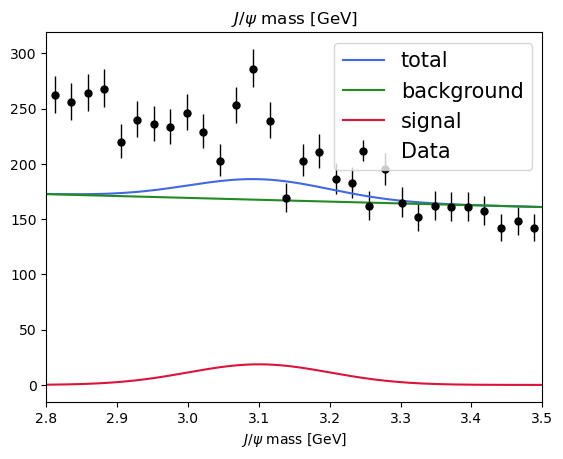
[10]:
def plot_fit(model, data, nbins=30, ax=None):
    # The function will be reused.
    if ax is None:
        ax = plt.gca()

    lower, upper = data.space.v1.limits

    # Creates and histogram of the data and plots it with mplhep.
    binneddata = data.to_binned(nbins)
    mplhep.histplot(binneddata, histtype="errorbar", yerr=True,
                    label="Data", ax=ax, color="black")

    binwidth = binneddata.space.binning[0].widths[0]  # all have the same width
    x = np.linspace(lower, upper, num=1000)

    # Line plots of the total pdf and the sub-pdfs.
    y = model.ext_pdf(x) * binwidth
    ax.plot(x, y, label="total", color="royalblue")
    for m, l, c in zip(model.get_models(), ["background", "signal"], ["forestgreen", "crimson"]):
        ym = m.ext_pdf(x) * binwidth
        ax.plot(x, ym, label=l, color=c)

    plt.xlabel(data.space.labels[0])
    ax.set_title(data.space.labels[0])
    ax.set_xlim(lower, upper)
    ax.legend(fontsize=15)

    return ax
[11]:
plot_fit(model, data) # before the fit
[11]:
<Axes: title={'center': '$J/\\psi$ mass [GeV]'}, xlabel='$J/\\psi$ mass [GeV]'>
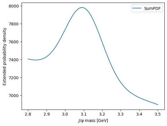
A quick plot
Sometimes, it’s useful to just quickly make a plot of the model without controlling all of the aspects. This can be done using the plot attribute of the model.
[12]:
model.plot.plotpdf()
/tmp/ipykernel_5189/4197811884.py:1: ExperimentalFeatureWarning: The function <function assert_initialized.<locals>.wrapper at 0x7fd20e1c67a0> is EXPERIMENTAL, potentially unstable and likely to change in the future! Use it with caution and feedback (Gitter, Mattermost, e-mail or https://github.com/zfit/zfit/issues) is very welcome!
  model.plot.plotpdf()
[12]:
<Axes: xlabel='$J/\\psi$ mass [GeV]', ylabel='Extended probability density'>
Loss
Since we have now the models and the datasets, we can e.g. pre-fit the signal PDF to the simulation.
[13]:
sig_nll = zfit.loss.UnbinnedNLL(sig_pdf, mc)
It warns us that we are using a non-extended loss. The extended loss also includes to fit the yield while the normal one does not. Since we want to fit the shape here only, we use the non-extended one.
[14]:
minimizer = zfit.minimize.Minuit(gradient="zfit")  # to use the analytic gradient. Set it to true will use the iminuit one
# minimizer = zfit.minimize.NLoptLBFGSV1()  # can be changed but maybe not as powerful as iminuit
# minimizer = zfit.minimize.ScipySLSQPV1()
[15]:
minimizer.minimize(sig_nll)
[15]:
FitResult of
<UnbinnedNLL model=[<zfit.<class 'zfit.models.dist_tfp.Gauss'>  params=[mu, sigma]] data=[<zfit.Data: Data obs=('Jpsi_M',) shape=(99032, 1)>] constraints=[]>
with
<Minuit Minuit tol=0.001>

╒═════════╤═════════════╤══════════════════╤═════════╤══════════════════════════════╕
│  valid  │  converged  │  param at limit  │   edm   │   approx. fmin (full | opt.) │
╞═════════╪═════════════╪══════════════════╪═════════╪══════════════════════════════╡
│  True   │    True     │      False       │ 5.2e-06 │         -275181.55 | -129185 │
╘═════════╧═════════════╧══════════════════╧═════════╧══════════════════════════════╛

Parameters
name      value  (rounded)    at limit
------  ------------------  ----------
mu                 3.09692       False
sigma            0.0150308       False
Fixing parameters
Sometimes we want to fix parameters obtained from MC, such as tailes. Here we will fix the sigma, just for demonstration purpose.
[16]:
sigma.floating = False
[17]:
nll = zfit.loss.ExtendedUnbinnedNLL(model, data)
[18]:
result = minimizer.minimize(nll)
[19]:
result
[19]:
FitResult of
<ExtendedUnbinnedNLL model=[<zfit.<class 'zfit.models.functor.SumPDF'>  params=[Composed_autoparam_1, Composed_autoparam_2]] data=[<zfit.Data: Data obs=('Jpsi_M',) shape=(6155, 1)>] constraints=[]>
with
<Minuit Minuit tol=0.001>

╒═════════╤═════════════╤══════════════════╤═════════╤══════════════════════════════╕
│  valid  │  converged  │  param at limit  │   edm   │   approx. fmin (full | opt.) │
╞═════════╪═════════════╪══════════════════╪═════════╪══════════════════════════════╡
│  True   │    True     │      False       │ 2.5e-05 │         -2362.59 |  9803.742 │
╘═════════╧═════════════╧══════════════════╧═════════╧══════════════════════════════╛

Parameters
name         value  (rounded)    at limit
---------  ------------------  ----------
bkg_yield             5991.64       False
sig_yield             163.073       False
lambda               -1.08982       False
mu                    3.09093       False
[20]:
result.hesse()  # calculate hessian error
result.errors()  # profile, using minos like uncertainty
print(result)
FitResult of
<ExtendedUnbinnedNLL model=[<zfit.<class 'zfit.models.functor.SumPDF'>  params=[Composed_autoparam_1, Composed_autoparam_2]] data=[<zfit.Data: Data obs=('Jpsi_M',) shape=(6155, 1)>] constraints=[]>
with
<Minuit Minuit tol=0.001>

╒═════════╤═════════════╤══════════════════╤═════════╤══════════════════════════════╕
│  valid  │  converged  │  param at limit  │   edm   │   approx. fmin (full | opt.) │
╞═════════╪═════════════╪══════════════════╪═════════╪══════════════════════════════╡
│  True   │    True     │      False       │ 2.5e-05 │         -2362.59 |  9803.742 │
╘═════════╧═════════════╧══════════════════╧═════════╧══════════════════════════════╛

Parameters
name         value  (rounded)        hesse               errors    at limit
---------  ------------------  -----------  -------------------  ----------
bkg_yield             5991.64  +/-      81  -     80   +     81       False
sig_yield             163.073  +/-      27  -     26   +     27       False
lambda               -1.08982  +/-   0.065  -  0.065   +  0.065       False
mu                    3.09093  +/-  0.0033  - 0.0033   + 0.0033       False
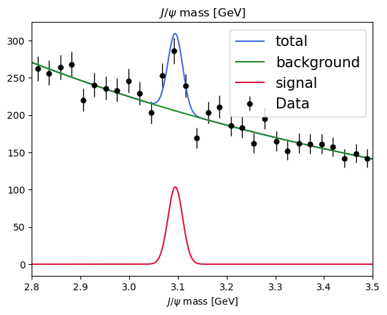
[21]:
plot_fit(model, data)
[21]:
<Axes: title={'center': '$J/\\psi$ mass [GeV]'}, xlabel='$J/\\psi$ mass [GeV]'>
Exercise: use hepstats to check the significance of our signal
[22]:
from hepstats.hypotests.calculators import AsymptoticCalculator
from hepstats.hypotests.parameters import POI

# the null hypothesis
sig_yield_poi = POI(sig_yield, 0)
calculator = AsymptoticCalculator(input=result, minimizer=minimizer)
/usr/share/miniconda/envs/analysis-essentials/lib/python3.11/site-packages/tqdm/auto.py:21: TqdmWarning: IProgress not found. Please update jupyter and ipywidgets. See https://ipywidgets.readthedocs.io/en/stable/user_install.html
  from .autonotebook import tqdm as notebook_tqdm
There is another calculator in hepstats called FrequentistCalculator which constructs the test statistic distribution \(f(q_{0} |H_{0})\) with pseudo-experiments (toys), but it takes more time.
The Discovery class is a high-level class that takes as input a calculator and a POI instance representing the null hypothesis, it basically asks the calculator to compute the p-value and also computes the signifance as
\begin{equation} Z = \Phi^{-1}(1 - p_0). \end{equation}
[23]:
from hepstats.hypotests import Discovery

discovery = Discovery(calculator=calculator, poinull=sig_yield_poi)
discovery.result()
[23]:
(np.float64(7.03648250777178e-12), np.float64(6.757152908419564))
Exercise play around! First things first: repeat the fit. The difference we will see is statistical fluctuation from the resampling of the data; we take only a fraction at random.
Change the fraction of data that we have, the BDT cut, the signal model…
Attention: it is easy to have a significance of inf here