7: Demonstration of distribution reweighting
Reweighting in HEP is used to minimize difference between real data and Monte-Carlo simulation.
Known process is used, for which real data can be obtained.
Target of reweighting: assign weights to MC such that MC and real data distributions coincide.
hep_ml.reweight contains methods to reweight distributions. Typically we use reweighting of monte-carlo to fight drawbacks of simulation, though there are many applications.
In this example we reweight multidimensional distibutions: original and target, the aim is to find new weights for original distribution, such that these multidimensional distributions will coincide.
Here we have a toy example without a real physics meaning.
Pay attention: equality of distibutions for each feature \(\neq\) equality of multivariate distributions.
All samples are divided into training and validation part. Training part is used to fit reweighting rule and test part is used to estimate reweighting quality.
[1]:
from xgboost import XGBClassifier

%matplotlib inline

import numpy as np
import pandas as pd
import uproot
from hep_ml import reweight
from matplotlib import pyplot as plt
Downloading data
[2]:
columns = ['hSPD', 'pt_b', 'pt_phi', 'vchi2_b', 'mu_pt_sum']

with uproot.open('https://starterkit.web.cern.ch/starterkit/data/advanced-python-2019/MC_distribution.root',
                            ) as original_file:
    original_tree = original_file['tree']
    original = original_tree.arrays(library='pd')
with uproot.open('https://starterkit.web.cern.ch/starterkit/data/advanced-python-2019/RD_distribution.root',
                          ) as target_file:
    target_tree = target_file['tree']
    target = target_tree.arrays(library='pd')
original_weights = np.ones(len(original))
prepare train and test samples
train part is used to train reweighting rule
test part is used to evaluate reweighting rule comparing the following things:
Kolmogorov-Smirnov distances for 1d projections
n-dim distibutions using ML (see below).
[3]:
from sklearn.model_selection import train_test_split

# divide original samples into training ant test parts
original_train, original_test = train_test_split(original)
# divide target samples into training ant test parts
target_train, target_test = train_test_split(target)

original_weights_train = np.ones(len(original_train))
original_weights_test = np.ones(len(original_test))
[4]:
from hep_ml.metrics_utils import ks_2samp_weighted

hist_settings = {'bins': 100, 'density': True, 'alpha': 0.7}


def draw_distributions(original, target, new_original_weights):
    plt.figure(figsize=[15, 7])
    for id, column in enumerate(columns, 1):
        xlim = np.percentile(np.hstack([target[column]]), [0.01, 99.99])
        plt.subplot(2, 3, id)
        plt.hist(original[column], weights=new_original_weights, range=xlim, **hist_settings)
        plt.hist(target[column], range=xlim, **hist_settings)
        plt.title(column)
        print('KS over ', column, ' = ', ks_2samp_weighted(original[column], target[column],
                                         weights1=new_original_weights, weights2=np.ones(len(target), dtype=float)))
Original distributions
KS = Kolmogorov-Smirnov distance: a measure of how well two distributions agree, the lower the distance, the better the agreement. In this case we want a low KS value.
[5]:
# pay attention, actually we have very few data
len(original), len(target)
[5]:
(1000000, 21441)
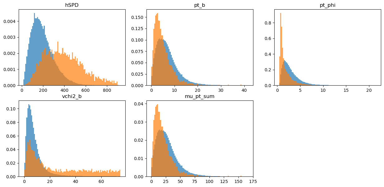
[6]:
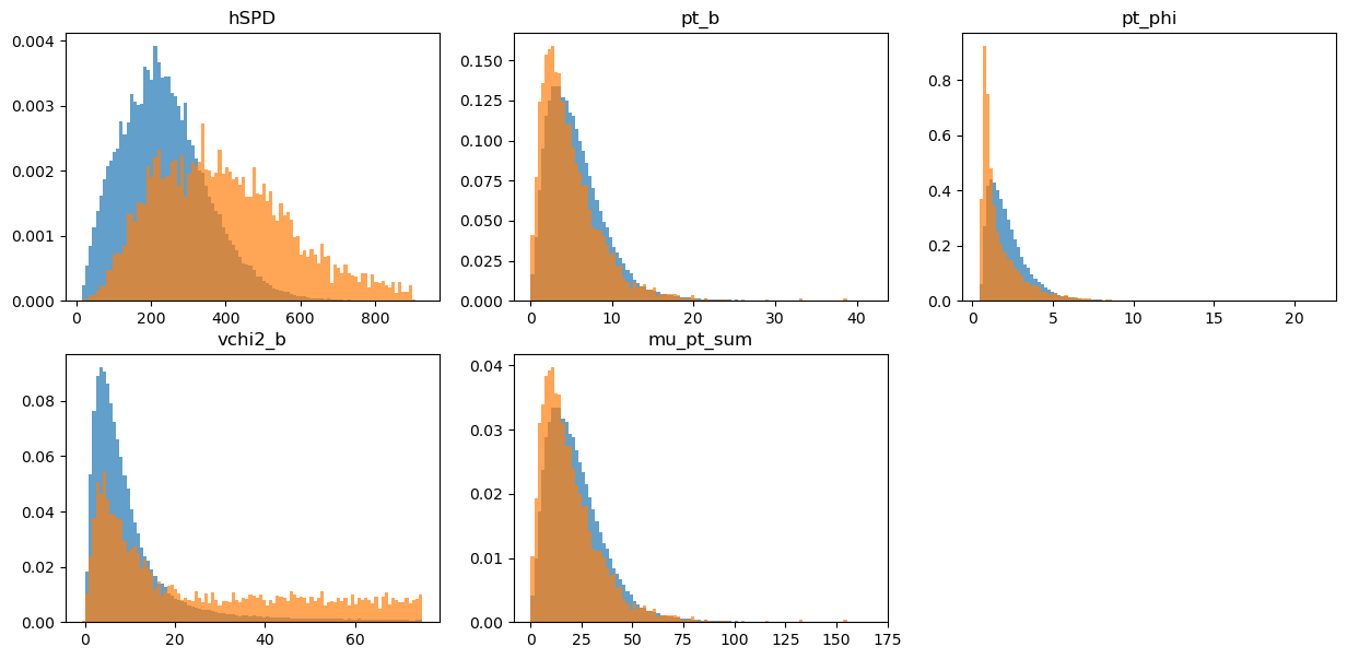
draw_distributions(original, target, original_weights)
KS over  hSPD  =  0.5203540728277889
KS over  pt_b  =  0.21639364439970188
KS over  pt_phi  =  0.4020113592414034
KS over  vchi2_b  =  0.40466385087324064
KS over  mu_pt_sum  =  0.21639364439970188
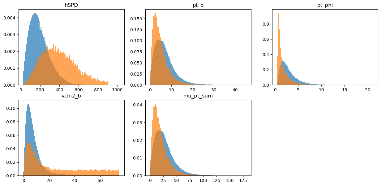
train part of original distribution
[7]:
draw_distributions(original_train, target_train, original_weights_train)
KS over  hSPD  =  0.5260418805970046
KS over  pt_b  =  0.2190009054713981
KS over  pt_phi  =  0.4005532238807191
KS over  vchi2_b  =  0.40391358208323225
KS over  mu_pt_sum  =  0.2190009054713981
test part for target distribution
[8]:
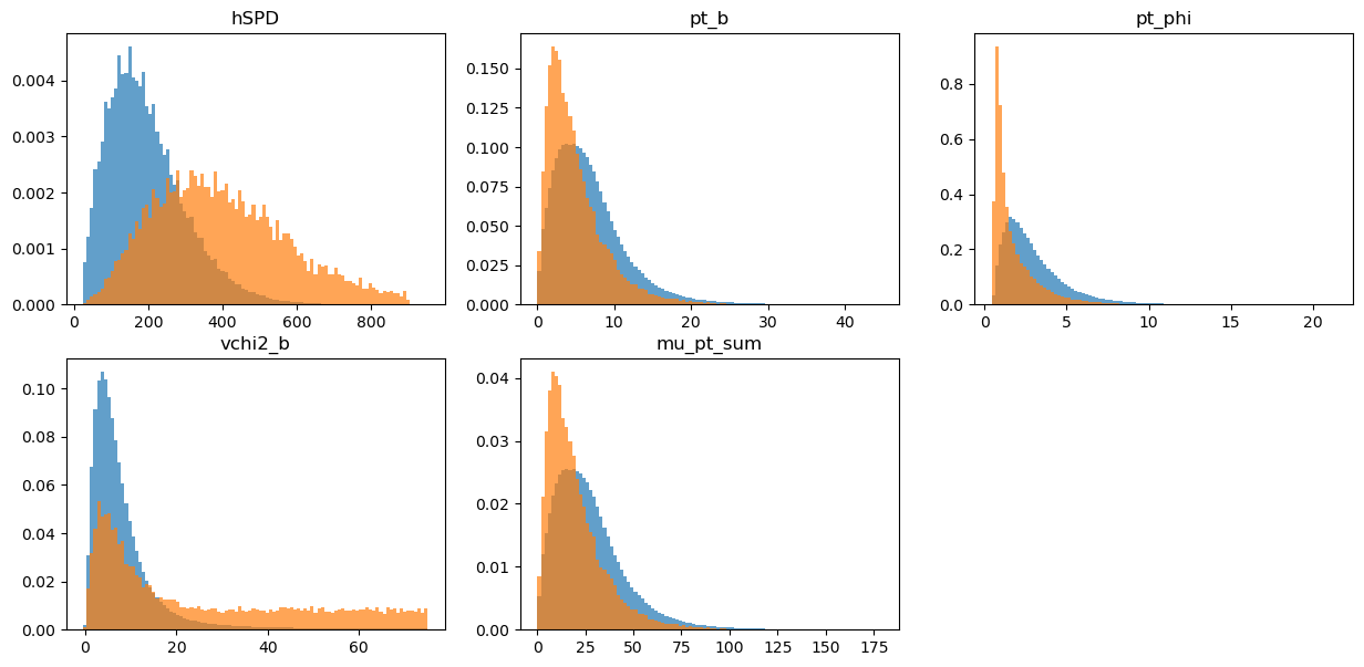
draw_distributions(original_test, target_test, original_weights_test)
KS over  hSPD  =  0.5064103074053462
KS over  pt_b  =  0.21115031038953475
KS over  pt_phi  =  0.4069045838461766
KS over  vchi2_b  =  0.40872052863349506
KS over  mu_pt_sum  =  0.21115031038953475
Bins-based reweighting in n dimensions
Typical way to reweight distributions is based on bins.
Usually histogram reweighting is used, in each bin the weight of original distribution is multiplied by:
\(m_{bin} = \frac{w_{target}}{w_{original}}\)
where \(w_{target}\) and \(w_{original}\) are the total weight of events in each bin for target and original distributions.
Simple and fast!
Very few (typically, one or two) variables
Reweighting one variable may bring disagreement in others
Which variable to use in reweighting?
[9]:
bins_reweighter = reweight.BinsReweighter(n_bins=20, n_neighs=1.)
bins_reweighter.fit(original_train, target_train)

bins_weights_test = bins_reweighter.predict_weights(original_test)
# validate reweighting rule on the test part comparing 1d projections
draw_distributions(original_test, target_test, bins_weights_test)
KS over  hSPD  =  0.40220194349142135
KS over  pt_b  =  0.11436596116021447
KS over  pt_phi  =  0.2858828314017112
KS over  vchi2_b  =  0.34873746771714065
KS over  mu_pt_sum  =  0.11436596116021447
Gradient Boosted Reweighter
This algorithm is inspired by gradient boosting and is able to fight curse of dimensionality. It uses decision trees and special loss functiion (ReweightLossFunction).
A classifier is trained to discriminate between real data and MC. This means we are able to reweight in several variables rather than just one. GBReweighter from hep_ml is able to handle many variables and requires less data (for the same performance).
GBReweighter supports negative weights (to reweight MC to splotted real data).
[10]:
reweighter = reweight.GBReweighter(n_estimators=50, learning_rate=0.1, max_depth=3, min_samples_leaf=1000,
gb_args={'subsample': 0.7})
reweighter.fit(original_train, target_train)
gb_weights_test = reweighter.predict_weights(original_test)
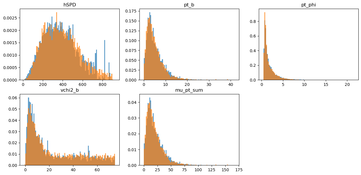
# validate reweighting rule on the test part comparing 1d projections
draw_distributions(original_test, target_test, gb_weights_test)
KS over  hSPD  =  0.033164189316626125
KS over  pt_b  =  0.02903464575744763
KS over  pt_phi  =  0.029009852859612772
KS over  vchi2_b  =  0.05908893529007331
KS over  mu_pt_sum  =  0.02903464575744763
Comparing some simple expressions:
The most interesting is checking some other variables in multidimensional distributions (those are expressed via original variables). Here we can check the KS distance in multidimensional distributions. (The lower the value, the better agreement of distributions.)
[11]:
def check_ks_of_expression(expression):
    col_original = original_test.eval(expression, engine='python')
    col_target = target_test.eval(expression, engine='python')
    w_target = np.ones(len(col_target), dtype='float')
    print('No reweight   KS:', ks_2samp_weighted(col_original, col_target,
                                                 weights1=original_weights_test, weights2=w_target))
    print('Bins reweight KS:', ks_2samp_weighted(col_original, col_target,
                                                 weights1=bins_weights_test, weights2=w_target))
    print('GB Reweight   KS:', ks_2samp_weighted(col_original, col_target,
                                                 weights1=gb_weights_test, weights2=w_target))
[12]:
check_ks_of_expression('hSPD')
No reweight   KS: 0.5064103074053462
Bins reweight KS: 0.40220194349142135
GB Reweight   KS: 0.033164189316626125
[13]:
check_ks_of_expression('hSPD * pt_phi')
No reweight   KS: 0.08513205260229018
Bins reweight KS: 0.11115639969557542
GB Reweight   KS: 0.021195130553905428
[14]:
check_ks_of_expression('hSPD * pt_phi * vchi2_b')
No reweight   KS: 0.36619022458566386
Bins reweight KS: 0.3333271483938009
GB Reweight   KS: 0.06834167572056049
[15]:
check_ks_of_expression('pt_b * pt_phi / hSPD ')
No reweight   KS: 0.46917148554361465
Bins reweight KS: 0.3742478736893725
GB Reweight   KS: 0.04486889975310382
[16]:
check_ks_of_expression('hSPD * pt_b * vchi2_b / pt_phi')
No reweight   KS: 0.498435370640539
Bins reweight KS: 0.4063515556745043
GB Reweight   KS: 0.06407035437469383
GB-discrimination
Let’s check how well a classifier is able to distinguish these distributions.
For this puprose we split the data into train and test, then we train a classifier to distinguish between the real data and MC distributions.
We can use the ROC Area Under Curve as a measure of performance. If ROC AUC = 0.5 on the test sample, the distibutions are identical, if ROC AUC = 1.0, they are ideally separable. So we want a ROC AUC as close to 0.5 as possible to know that we cannot separate the reweighted distributions.
[17]:
from sklearn.metrics import roc_auc_score
from sklearn.model_selection import train_test_split
from xgboost import XGBClassifier

data = np.concatenate([original_test, target_test])
labels = np.array([0] * len(original_test) + [1] * len(target_test))

weights = {}
weights['original'] = original_weights_test
weights['bins'] = bins_weights_test
weights['gb_weights'] = gb_weights_test


for name, new_weights in weights.items():
    W = np.concatenate([new_weights / new_weights.sum() * len(target_test), [1] * len(target_test)])
    Xtr, Xts, Ytr, Yts, Wtr, Wts = train_test_split(data, labels, W, random_state=42, train_size=0.51)
    clf = XGBClassifier(subsample=0.8, n_estimators=50).fit(Xtr, Ytr, sample_weight=Wtr)

    print(name, roc_auc_score(Yts, clf.predict_proba(Xts)[:, 1], sample_weight=Wts))
original 0.9254028623600775
bins 0.8986668467440414
gb_weights 0.5678748722490807
Great!
To the classifier, the two datasets seem now nearly undistingishable. Can we improve that? The GBReweighter is quite sensible to its hyperparameters, especially to n_estimators. Feel free to go back and increase it (to e.g. 250). What happens?
Answer: we get an even lower score! 0.49! Yeey! Or wait…
What did just happen?
Our algorithm completely overfitted the distribution. The problem is that while for the classification we have a true label for each event, we do not have a true weight for each event, we just have a true distribution so a “true local density” of the events. Or something like that.
As powerful as the GBReweighter is, as much does it need some care to be taken when choosing the hyperparameters as it can easily overfit. And, worse, the overfitting cannot be spotted so easily.
While this is a topic on its own, whatever you do with the GBReweighter, be sure to really validate your result.
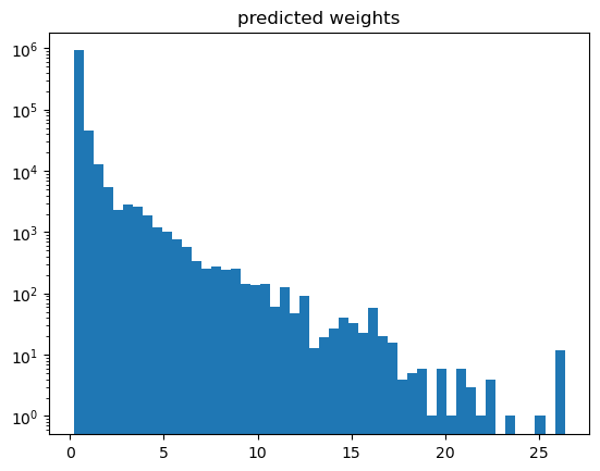
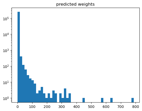
A hint of what may goes wrong is given when plotting the weights.
[18]:
plt.hist(weights['gb_weights'], bins=50)
plt.yscale('log')
plt.title('predicted weights')
[18]:
Text(0.5, 1.0, 'predicted weights')
[19]:
np.max(weights['gb_weights']), np.sum(weights['gb_weights'])
[19]:
(np.float64(682.0773551690282), np.float64(68408.55687929984))
With such a high weight for a single event, this does not look desireable. And be aware of ad-hoc solutions: just clipping or removing weights is completely wrong as this would disturb the distribution completely.
A good way to proceed is to play around with the hyperparameters in order to avoid overfitting until the weights distribution looks “reasonable”. Especially we don’t want to have high weights in there if avoidable.
How to tune
First find an appropriate number of estimators.
max_depth basically determines the order of correlations to be taken into account.
n_estimators has a tradeoff vs learning_rate. Increasing the former by a factor of n and reducing the latter by a factor of 1 / n keeps the reweighter with the same capability (e.g. overfitting) but tends to smooth out things. So use this at the end as more estimators take more time.
Folding reweighter
FoldingReweighter uses k folding in order to obtain unbiased weights for the whole distribution.
The hyperparameters have been adjusted here. Be aware that n_estimators=80 with learning_rate=0.01 reads as n_estimators=8 and learning_rate=0.1 (in the above). So we greatly reduced the number of estimators.
[20]:
# define base reweighter
reweighter_base = reweight.GBReweighter(n_estimators=40,
learning_rate=0.02, max_depth=4, min_samples_leaf=100,
gb_args={'subsample': 0.8})
reweighter = reweight.FoldingReweighter(reweighter_base, n_folds=2)
# it is not needed divide data into train/test parts; reweighter can be train on the whole samples
reweighter.fit(original, target)
# predict method provides unbiased weights prediction for the whole sample
# folding reweighter contains two reweighters, each is trained on one half of samples
# during predictions each reweighter predicts another half of samples not used in training
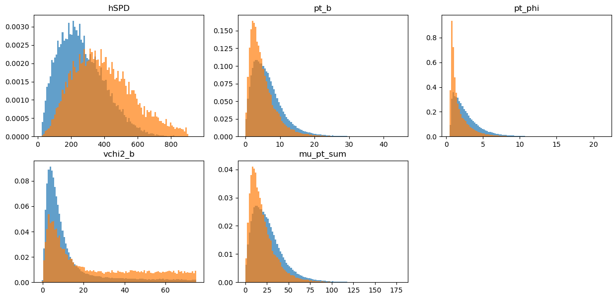
folding_weights = reweighter.predict_weights(original)
draw_distributions(original, target, folding_weights)
KFold prediction using folds column
KS over  hSPD  =  0.3064090606205577
KS over  pt_b  =  0.18039052436075925
KS over  pt_phi  =  0.30777785918417755
KS over  vchi2_b  =  0.29748251583601615
KS over  mu_pt_sum  =  0.18039052436075925
GB discrimination for reweighting rule
[21]:
data = np.concatenate([original, target])
labels = np.array([0] * len(original) + [1] * len(target))

weights = {}
weights['original'] = original_weights
weights['2-folding'] = folding_weights


for name, new_weights in weights.items():
    W = np.concatenate([new_weights / new_weights.sum() * len(target), [1] * len(target)])
    Xtr, Xts, Ytr, Yts, Wtr, Wts = train_test_split(data, labels, W, random_state=42, train_size=0.51)
    clf = XGBClassifier(subsample=0.6, n_estimators=30).fit(Xtr, Ytr, sample_weight=Wtr)

    print(name, roc_auc_score(Yts, clf.predict_proba(Xts)[:, 1], sample_weight=Wts))
original 0.9351539768528147
2-folding 0.8271247564689598
[22]:
plt.hist(weights['2-folding'], bins=50)
plt.yscale('log')
plt.title('predicted weights')
[22]:
Text(0.5, 1.0, 'predicted weights')