Introduction
Overview
Teaching: 10 min
Exercises: 0 minQuestions
Why Python?
What is Uproot?
Why should I use it?
Objectives
Explain some advantages of Python and Uproot.
Python and HEP
For quite a while now, ROOT has been the main software used by particle physicists for data analysis. ROOT is written in C++, and at least until recently most analysis code has also been written in C++. Outside of HEP, Python is a more commonly used language for data analysis, which means that there are many popular and well-supported tools that can be utilized for common tasks. Python is also generally considered easier to learn than C++.
Uproot
Uproot is a Python module that can read and write files in the ROOT format. It’s part of the Scikit-HEP project, a collection of Python tools for HEP data analysis. Uproot isn’t the only way to read/write ROOT files in Python; there are other packages that allow you to do this. However, there are some significant advantages of Uproot. We’ll go through a few here.
Minimal dependencies
The only software required by Uproot (other than Python itself, of course) is NumPy.
NumPy is by far the most popular Python package for handling arrays of data.
It’s included in the Anaconda distribution by default, and in general most people using Python for any kind of data analysis will probably already have it installed.
Awkward Array and Vector are not required but highly recommended for use with Uproot.
Uproot, Awkward Array, and Vector are all part of the Scikit-HEP project.
All of the above are Python modules, which can be installed with nothing more than pip or conda.
Most importantly, Uproot does not require any part of the ROOT software, which is quite large and can be non-trivial to install properly.
Speed
Uproot was designed for efficient reading of files. It uses NumPy for operations on data, which calls compiled vectorized functions to perform very fast calculations on arrays.
When you import a Python package that uses ROOT, there can be a delay of several seconds while all of the required libraries are loaded. This is required every time you restart the Python interpreter or run a script. By virtue of not using ROOT itself, Uproot doesn’t have this issue.
Jagged arrays
One issue with manipulating HEP data in Python is that it is often not rectangular. That is, the length of object collections is not constant. For example, different events will have different numbers of jets, and different jets will have different numbers of associated tracks. Such arrays are called jagged arrays. Packages like NumPy are only designed to work with rectangular arrays, where each dimension has a fixed length throughout the entire array.
Jagged vs. rectangular arrays
The name “jagged array” comes from the idea that if you have a 2D array in which there’s a different number of entries in each row and you line rows up by their first element, then the right edge of the array will be “jagged” as opposed to straight:
Rectangular array:
[[0, 1],
 [2, 3],
 [4, 5],
 [6, 7],
 [8, 9]]
Jagged array:
[[0, 1],
 [2, 3, 4],
 [5],
 [6, 7],
 [8, 9]]
Awkward Array is a package used to deal with jagged arrays so that they can be manipulated in ways almost identical to standard rectangular NumPy arrays. Other Python packages for reading ROOT files usually do not support jagged arrays, which means that you cannot do operations on multiple events at once if you have jagged data. But Uproot and Awkward Array can, and this is generally much faster than operating on one event at a time. We’ll come back to this topic in the “Columnar Analysis” section.
Key Points
Uproot is a fast and lightweight Python package for reading and writing ROOT files.
Uproot is designed to work efficiently with jagged arrays of data.
Opening files
Overview
Teaching: 20 min
Exercises: 0 minQuestions
How do I open a ROOT file with Uproot?
How can I tell what’s in the file?
How do I access the contents?
Objectives
Open a ROOT file and list its contents.
Access objects within a ROOT file.
Example motivation
In order to learn how to use Uproot, we’ll try to do a very short and simple analysis to look for resonances in a dimuon events. The example ROOT file is from real CMS data during proton-proton collisions in 2012. Make sure you’ve downloaded it from the Setup page and put it in your working directory. Our first goal is just to get to the data within Uproot, so we need to open the file and navigate to the muon information.
Opening a file
The first thing you must do whenever you want to use Uproot is import it, just like any other Python module:
import uproot
Import errors?
If you get something like:
Traceback (most recent call last):
  File "<stdin>", line 1, in <module>
ModuleNotFoundError: No module named 'uproot'
then this means Uproot hasn’t been installed properly. Check the Setup page for detailed instructions. If you’re using
conda(like Anaconda or Miniconda), make sure you’ve activated the same environment where you installed Uproot.
Now open the ROOT file and assign it to a variable (which I’ve named file here):
file = uproot.open('uproot-tutorial-file.root')
If you inspect file, you can see that it’s a ReadOnlyDirectory object:
file
<ReadOnlyDirectory '/' at 0x(some hexadecimal number here)>
File contents
Just like any other kind of directory, you can list the contents (of the file). The name of each item in the file is called a “key”.
file.keys()
['Events;1']
We can see that there is one key: “Events”. This doesn’t tell us what kind of object it refers to, though. ROOT files can contain many different types of objects, including subdirectories. The following function provides a way to inspect the types of each item:
file.classnames()
{'Events;1': 'TTree'}
The output contains pairs of the form name: type.
Therefore the key Events refers to a TTree object.
This is where all the data in this file is stored.
Why the
;1?You may be wondering why there’s a
;1after “Events”. This notation refers to the cycle number, which is a detail of the ROOT file format that we don’t need to care about. This;1shows up if you open the file in ROOT itself as well.
Accessing contents
Now we want to actually access the object inside the file. You can do this just as you would to get an item in an array:
file['Events']
<TTree 'Events' (6 branches) at 0x(hexadecimal number)>
This expression refers to the actual TTree object, which we will look at next.
Key Points
Opening and navigating files in Uproot isn’t that different from doing so in ROOT.
Use
.keys()to see the contents of a file.Use the form
file['key']to access an object inside a file.
Trees, Branches, and Events
Overview
Teaching: 20 min
Exercises: 5 minQuestions
How do I access a TTree?
How can I tell what branches are in a TTree?
How do I read the data from a TTree?
Objectives
List the branches in a tree.
Access the branches in a tree.
Create a table from tree branches.
Access data for a particular event.
Trees
Trees in ROOT are basically just tables of information. Trees are composed of branches, which are the columns of the table. The rows usually represent events (individual bunch crossings).
First we assign the tree to a variable (named tree here)
tree = file['Events']
In order to find out what information is in the tree, we need to know what the branches (columns) are.
The term key is used (again) here to refer to the names of the branches.
tree.keys()
['nMuon', 'Muon_pt', 'Muon_eta', 'Muon_phi', 'Muon_mass', 'Muon_charge']
The above output is a list of the branch names.
So we can see that for each event, we will have the number of muons in the event (nMuon) and the pT, eta, phi, mass, and charge of each muon.
But how do we get the actual data from the table? There are several ways with Uproot, but the simplest is with the arrays() function:
tree.arrays()
<Array [{nMuon: 2, Muon_pt: [10.8, ... -1, 1]}] type='100000 * {"nMuon": uint32,...'>
You can see some numbers in there, which indeed are from the data in the tree.
Branches
Now we assign this object (which contains both the names and contents of the branches) to another variable (branches):
branches = tree.arrays()
Next let’s just look at each branch individually.
You can access a single branch from branches in a similar way to getting an item from a ROOT file object (array-like notation):
branches['nMuon']
<Array [2, 2, 1, 4, 4, 3, ... 0, 3, 2, 3, 2, 3] type='100000 * uint32'>
You can see the partial list of numbers in the output that represents the number of muons in each event.
It’s abbreviated with an ellipsis (...) so that it doesn’t take up the whole page.
Error?
If you get something like:
Traceback (most recent call last):
  File "<stdin>", line 1, in <module>
KeyError: 'nMuon'
then you are almost certainly using an older version of Uproot that is not compatible with the rest of this tutorial. If this is the case, install the latest version of Uproot, restart the notebook’s kernel, and try again.
These Array objects are a special type provided by the Awkward Array package.
The type=100000 * uint32 means that there are 100,000 entries and that each entry is a 32-bit unsigned integer. Each entry corresponds to one event.
Let’s look at another branch:
branches['Muon_pt']
<Array [[10.8, 15.7], ... 11.4, 3.08, 4.97]] type='100000 * var * float32'>
This is a jagged array because the number of entries is different for different events (because each event can have a different number of muons).
Note that there are square brackets [] surrounding the list of entries for each event.
The type='100000 * var * float32' means that there are 100,000 rows, each containing a variable number of 32-bit floating point numbers.
This is basically an array of arrays (or a 2D array).
Events
If we want to focus on a particular event, we can index it just like a normal array:
branches['Muon_pt'][0]
<Array [10.8, 15.7] type='2 * float32'>
From the above output, the first event has two muons, and the two numbers in the list are the muons’ pT. It’s not specified anywhere in the file, but the units are GeV. Let’s look at the third event:
branches['Muon_pt'][2]
<Array [3.28] type='1 * float32'>
It only has one muon.
Exercise
Print out the pT of all muons that are in only the first 10 events. (There are many possible ways to do this.)
Solution
Here’s one way to do it. All that matters is that you get the same numbers (and number of numbers) in the output
for i in range(10):
    print(branches['Muon_pt'][i])
[10.8, 15.7] [10.5, 16.3] [3.28] [11.4, 17.6, 9.62, 3.5] [3.28, 3.64, 32.9, 23.7] [3.57, 4.57, 4.37] [57.6, 53] [11.3, 23.9] [10.2, 14.2] [11.5, 3.47]
What if we want to get all of the information about a single event?
So far we’ve accessed data in branches by providing a branch name, but we can also just use an event index:
branches[0]
<Record ... 0.106], Muon_charge: [-1, -1]} type='{"nMuon": uint32, "Muon_pt": va...'>
This is a Record object, which is another special type provided by Awkward Array.
It functions basically the same way as a standard Python dictionary (dict).
Unfortunately, most of the interesting information is still hidden in the above output to save space.
A little trick we can use to force printing all the data is adding .tolist():
branches[0].tolist()
{'nMuon': 2,
 'Muon_pt': [10.763696670532227, 15.736522674560547],
 'Muon_eta': [1.0668272972106934, -0.563786506652832],
 'Muon_phi': [-0.03427272289991379, 2.5426154136657715],
 'Muon_mass': [0.10565836727619171, 0.10565836727619171],
 'Muon_charge': [-1, -1]}
There we go. Now we can see the whole picture for an individual event.
.tolist()
.tolist()is a NumPy function that has been extended to Awkward Array objects. As the name suggests, it converts NumPy arrays to Python lists. In the case of trees, which have named branches, it actually converts to a dictionary of lists. It can be very useful when you want to understand exactly what’s in anArrayorRecord. Be careful when using it, though–trying to print out an entire branch or tree could cause Python to crash if it’s large enough. Therefore it’s best to only usetolist()on one or a few events at a time to be safe.
Key Points
TTrees are tables of data.
Trees are made of branches, which are columns in the table.
Each row represents an event.
Histograms
Overview
Teaching: 20 min
Exercises: 5 minQuestions
How do I make a histogram in Python (without ROOT)?
How can I change histogram settings?
Objectives
Create a histogram of an array (regular or jagged).
Make a histogram’s axes logarithmic.
Histogramming basics
Histograms are the most important type of plots for particle physics. We’ll need to know how to make them with the tools we have. Matplotlib is the standard and most popular plotting package for Python, and it is quite powerful, so we’ll use it. First we import it:
import matplotlib.pyplot as plt
(It’s customary to import it abbreviated as plt as above, which saves some typing.)
The histogram function in Matplotlib is hist().
We can see what it does by just passing it our nMuon branch:
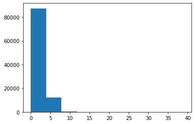
plt.hist(branches['nMuon'])
(array([8.7359e+04, 1.2253e+04, 3.5600e+02, 2.8000e+01, 2.0000e+00,
        1.0000e+00, 0.0000e+00, 0.0000e+00, 0.0000e+00, 1.0000e+00]),
 array([ 0. ,  3.9,  7.8, 11.7, 15.6, 19.5, 23.4, 27.3, 31.2, 35.1, 39. ]),
 <a list of 10 Patch objects>)
What’s with all the numbers above the plot?
hist()actually returns all the bin contents and bin edges in case you want to do something with them after creating the plot. We don’t need these return values, and they clutter up the notebook, so we should get rid of them. There are a few ways to do this, but I think the best practice is to addplt.show(), which is a way to tell Matplotlib when your plot is all set up and ready to be displayed. As a consequence ofhist()not being the last line in the notebook cell, the bin values will no longer be printed. For example:plt.hist(branches['nMuon']) plt.show()I’ll follow this convention from now on.
That created a histogram, but it’s not a very good one.
You can’t really understand much about the distribution because the binning and scale are too large.
These settings are controlled by the bins and range parameters:
plt.hist(branches['nMuon'], bins=10, range=(0, 10))
plt.show()
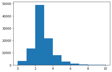
bins here is the total number of bins (of equal width), and range is a pair of numbers representing where the first bin starts and where the last bin ends.
Binning and range tips
Getting the binning and range right for a histogram is somewhat of an art, but I often find it helpful to know the mean, standard deviation, minimum, and maximum of the original distribution.
First, import NumPy via:
import numpy as npThen the following functions calculate these values for an array:
np.mean(branches['nMuon'])2.35286np.std(branches['nMuon'])1.19175912851549np.min(branches['nMuon'])0np.max(branches['nMuon'])39
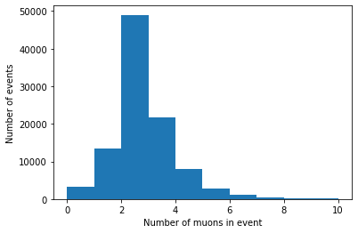
Hmm, we’re still missing axis titles on the histogram.
(Always label your plots!)
We can do this with the xlabel() and ylabel() functions:
plt.hist(branches['nMuon'], bins=10, range=(0, 10))
plt.xlabel('Number of muons in event')
plt.ylabel('Number of events')
plt.show()
Histogramming a jagged array
We can make histograms of the other branches as well, but there’s one more step necessary because of their jaggedness. Matplotlib expects a series of data to be in a 1D array, so we need to convert or flatten the jagged 2D array into a 1D array. In order to do this, we need to import Awkward Array:
import awkward as ak
Then use ak.flatten() on the branch’s array:
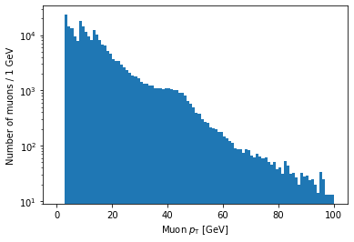
plt.hist(ak.flatten(branches['Muon_pt']), bins=100, range=(0, 100))
plt.xlabel('Muon $p_{\mathrm{T}}$ [GeV]')
plt.ylabel('Number of muons / 1 GeV')
plt.show()
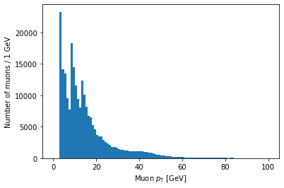
Note that you can use LaTeX in Matplotlib labels (as I did above).
Logarithmic scales
Another important thing to know is how to set axes to a logarithmic scale.
For the y-axis, this is as simple as adding a line with plt.yscale('log'):
plt.hist(ak.flatten(branches['Muon_pt']), bins=100, range=(0, 100))
plt.xlabel('Muon $p_{\mathrm{T}}$ [GeV]')
plt.ylabel('Number of muons / 1 GeV')
plt.yscale('log')
plt.show()
As you might guess, plt.xscale('log') will make the x-axis scale logarithmic.
The issue is that this doesn’t make the bin sizes logarithmic, so the plot will end up looking quite strange in most cases.
The solution to this is to use a NumPy function called logspace to calculate logarithmic bin edges:
import numpy as np
plt.hist(ak.flatten(branches['Muon_pt']), bins=np.logspace(np.log10(1), np.log10(100), 100))
plt.xlabel('Muon $p_{\mathrm{T}}$ [GeV]')
plt.xscale('log')
plt.ylabel('Number of muons')
plt.show()
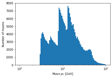
In the above example, bins is being set to an array.
If Matplotlib sees that bins is an array, it will use the values of the array to set the bin edges rather than try to evenly space them across range.
Don’t worry too much if this seems confusing; the details of how this works isn’t important for this lesson.
The important part is that, inside the logspace() call, you can modify the numbers to change where the bins start and end and how many bins there are.
Don’t remove the np.log10 part, though.
Exercise
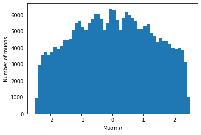
Make a histogram of the eta of all muons. Play around with the options described in this page to try to get a nice looking plot.
Solution
Your plot might look a bit different, but it’s fine as long as the binning is reasonable such that you can see the same distribution features.
plt.hist(ak.flatten(branches['Muon_eta']), bins=50, range=(-2.5, 2.5))
plt.xlabel('Muon $\eta$')
plt.ylabel('Number of muons')
plt.show()
Key Points
Use the
binsand/orrangeparameters to improve histogram binning.Make sure your axes are labeled.
Jagged arrays must be flattened before histogramming.
Columnar Analysis
Overview
Teaching: 25 min
Exercises: 5 minQuestions
What is columnar analysis?
What are its advantages over row-based analysis?
How do I perform selections and operations on columns?
Objectives
Count items passing some selection criteria.
Apply selection criteria to get passing events/objects.
Plot different selections for comparison.
Uproot is designed for columnar analysis, which means performing operations on entire columns (branches) at a time, rather than operating on every event individually.
Counting
The simplest task we need for analysis is counting (i.e., cutflow).
To count the total number of events, we can use the Python built-in function len() on any of the following:
len(branches)
len(branches['nMuon'])
len(branches['Muon_pt']) # or any of the other branches...
100000
So there are 100,000 events.
Exercise
Note that this is not the total number of muons, despite running
len()on a branch that has a number for every single muon (Muon_pt)! Why is this? Can you write some code that does give the total number of muons in the file?Solution
len()only looks at the length along the first dimension of the array.Muon_ptis a 2D array. In order to count every muon individually, we need to flatten the array to 1D.len(ak.flatten(branches['Muon_pt']))235286
Selections
Selections from 1D arrays
To do more interesting counting or plotting, we want to be able to select only events or muons that pass some criteria.
Just as you can compare two numbers, like 1 < 2 and get a True or False value, you can put arrays in comparisons as well.
Let’s look at this case:
branches['nMuon'] == 1
<Array [False, False, True, ... False, False] type='100000 * bool'>
This is checking for equality between an array and the number 1.
Of course these are different types (array vs. scalar), so the Python objects are certainly not identical, but you can see the return value is not just False.
What happens is that each element in the array is compared to the scalar value, and the return value is a new array (of the same shape) filled with all these comparison results.
So we can interpret the output as the result of testing whether each event has exactly one muon or not.
The first two events do not, the third does, and so on.
This array of Boolean values is called a mask because we can use it to pick out only the elements in the array that satisfy some criteria (like having exactly one muon). This is very useful, and we will save it to a variable to save typing later:
single_muon_mask = branches['nMuon'] == 1
Counting with selections
Now let’s say we want to know how many of these single-muon events there are.
Note that len() won’t work because the length of the array is still 100,000.
That is, there’s a value for every event (even if that value is False).
We need the number of Trues in the array.
There are multiple ways to do this, but my favorite is:
np.sum(single_muon_mask)
13447
sum() adds all the array values together.
True is interpreted as 1 and False is interpreted as 0, thus sum() is just the number of True entries.
So there are 13,447 events with exactly one muon.
Applying a mask to an array
If we want to apply some selection to an array (i.e., cut out events or muons that don’t pass), we just act like the selection mask is an index. For example, if we want the pT of only those muons in events with exactly one muon (so they’re the only muon in that event):
branches['Muon_pt'][single_muon_mask]
<Array [[3.28], [3.84], ... [13.3], [9.48]] type='13447 * var * float32'>
We can check that we really are only looking at the events that pass the selection by looking the number of rows:
len(branches['Muon_pt'][single_muon_mask])
13447
Yep, this matches the counting from single_muon_mask.sum() above.
Plotting with selections
We can also use masks to plot quantities after some selection. For example, let’s plot the muon pT for only the single-muon events:
plt.hist(ak.flatten(branches['Muon_pt'][single_muon_mask]), bins=100, range=(0, 100))
plt.xlabel('Muon $p_{\mathrm{T}}$ [GeV]')
plt.ylabel('Number of single muons / 1 GeV')
plt.yscale('log')
plt.show()
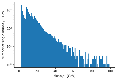
If you’re looking carefully, you might notice that this plot is missing the hump around 45 GeV that was in the pT plot before (for all muons). We accidentally ran into a hint of an effect from real physics. Neat!
Selections from a jagged array
Let’s look at a comparison for a jagged array, using the absolute value of muon eta:
eta_mask = abs(branches['Muon_eta']) < 2
eta_mask
<Array [[True, True], ... True, True, True]] type='100000 * var * bool'>
Again, the mask array has the same dimensions as the original array. There’s one Boolean value for each muon, corresponding to whether its eta is less than 2 in absolute value.
Counting
We can do counting and plotting just as before:
np.sum(eta_mask)
204564
This is the number of muons that pass the eta cut.
Plotting
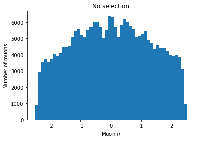
Let’s plot both the original eta distribution and the one after the cut to verify its effect:
plt.hist(ak.flatten(branches['Muon_eta']), bins=50, range=(-2.5, 2.5))
plt.title('No selection')
plt.xlabel('Muon $\eta$')
plt.ylabel('Number of muons')
plt.show()

plt.hist(ak.flatten(branches['Muon_eta'][eta_mask]), bins=50, range=(-2.5, 2.5))
plt.title('With $|\eta| < 2$ selection')
plt.xlabel('Muon $\eta$')
plt.ylabel('Number of muons')
plt.show()
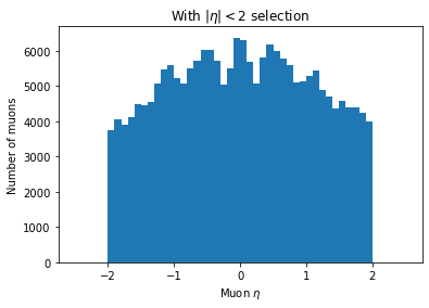
You can see the second plot just has both ends past 2 cut off, demonstrating that we’ve cut those muons out.
Operations on selections
We can invert selections with ~ (the NOT operator):
~single_muon_mask
<Array [True, True, False, ... True, True] type='100000 * bool'>
This new mask is False only for events with exactly one muon and True otherwise.
We can get the intersection of selections with & (the AND operator):
single_muon_mask & eta_mask
<Array [[False, False], ... False, False]] type='100000 * var * bool'>
This mask is True only for muons with no other muons in their event and abs(eta) < 2.
Or we can get the union of selections with | (the OR operator):
single_muon_mask | eta_mask
<Array [[True, True], ... True, True, True]] type='100000 * var * bool'>
This mask is True for muons which are the only muon in their event or which have abs(eta) < 2.
Warning about combining selections
You have to be careful about combining comparisons with the operators above. Consider the following expression:
False == False & FalseTrueIt’s a common mistake to assume that this expression would be
Falseby interpreting it as:(False == False) & FalseFalseThe issue is that
&has a higher precedence than==, so the first expression is actually equivalent to:False == (False & False)TrueWhat this means is that parentheses are necessary for expressions like this to have the correct meaning:
(branches['nMuon'] == 1) & (abs(branches['Muon_eta']) < 2)
Comparing histograms
Now we can use these operations to compare distributions for different selections.
Let’s look at the pT of single-event muons split into two groups by whether or not abs(eta) < 2.
All we have to do is provide a list of arrays as the first argument to hist rather than just one array.
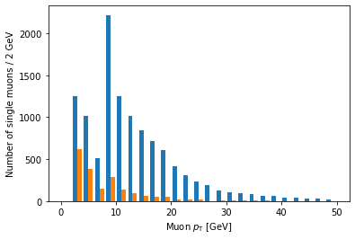
Note the square brackets around the two arrays:
plt.hist([ak.flatten(branches['Muon_pt'][single_muon_mask & eta_mask]),
          ak.flatten(branches['Muon_pt'][single_muon_mask & ~eta_mask])],
         bins=25, range=(0, 50))
plt.xlabel('Muon $p_{\mathrm{T}}$ [GeV]')
plt.ylabel('Number of single muons / 2 GeV')
plt.show()
Ah, but it doesn’t actually say which histogram is which. For that, we need to add labels and a legend:
plt.hist([ak.flatten(branches['Muon_pt'][single_muon_mask & eta_mask]),
          ak.flatten(branches['Muon_pt'][single_muon_mask & ~eta_mask])],
         label=['$|\eta| < 2$', '$|\eta| \geq 2$'],
         bins=25, range=(0, 50))
plt.xlabel('Muon $p_{\mathrm{T}}$ [GeV]')
plt.ylabel('Number of single muons / 2 GeV')
plt.legend()
plt.show()
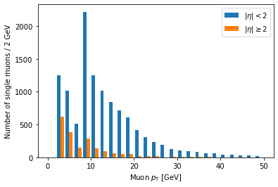
label is a list of strings passed to hist, corresponding to the arrays (in the same order),
and we have to add plt.legend() in order to actually draw a legend with those labels.
Another problem is that these histograms are on different scales because there are fewer large eta muons.
Often we want to compare only the shapes of the distribution, so we normalize the integral of each to 1.
We can achieve this by adding density=True to the hist() call:
plt.hist([ak.flatten(branches['Muon_pt'][single_muon_mask & eta_mask]),
          ak.flatten(branches['Muon_pt'][single_muon_mask & ~eta_mask])],
         label=['$|\eta| < 2$', '$|\eta| \geq 2$'],
         bins=25, range=(0, 50), density=True)
plt.title('Normalized')
plt.xlabel('Muon $p_{\mathrm{T}}$ [GeV]')
plt.ylabel('Number of single muons / 2 GeV')
plt.legend()
plt.show()
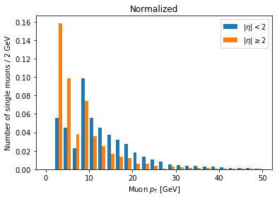
Now we can clearly see there’s a significantly higher fraction of muons with abs(eta) >= 2 at lower pT compared to muons with abs(eta) < 2. This makes geometric sense, since muons at higher abs(eta) are traveling in a direction less perpendicular to the beam.
(This name of the density parameter refers to the idea of interpreting the histogram as a probability density function, which always has an integral of 1.)
Columnar vs. row-based analysis
As an aside about columnar analysis, take a look at this comparison of speed for counting muons with abs(eta) < 2.
The first example is a row-based approach, using
forloops over every event and every muon in the event:%%time eta_count = 0 for event in branches['Muon_eta']: for eta in event: if abs(eta) < 2: eta_count += 1 eta_countCPU times: user 4.78 s, sys: 77.2 ms, total: 4.86 s Wall time: 4.88 s 204564The next example uses columnar operations, running on all muons at once:
%%time

np.sum(abs(branches['Muon_eta']) < 2)
CPU times: user 5.18 ms, sys: 1 ms, total: 6.18 ms Wall time: 4.87 ms 204564The columnar approach here is about 1000 times faster.
Key Points
Selections are created by comparisons on arrays and are represented by masks (arrays of Boolean values).
Selections are applied by acting like a mask is an array index.
Avoid
forloops whenever possible in analysis (especially in Python).
Getting Physics-Relevant Information
Overview
Teaching: 20 min
Exercises: 10 minQuestions
How can I use columnar analysis to do something useful for physics?
Objectives
Find dimuon invariant mass resonances.
Okay, we’re finally ready to look for resonances in dimuon events.
We need a mask that selects events with exactly two muons:
two_muons_mask = branches['nMuon'] == 2
Now we need to construct the four-momenta of each muon.
Vector is a package that provides an interface to operate on 2D, 3D, and 4D vectors.
We can get the four-momenta of all muons in the tree by using vector.zip and passing it the pT, eta, phi, and mass arrays:
import vector
muon_p4 = vector.zip({'pt': branches['Muon_pt'], 'eta': branches['Muon_eta'], 'phi': branches['Muon_phi'], 'mass': branches['Muon_mass']})
We’ll go ahead and filter out events that don’t contain exactly two muons:
two_muons_p4 = muon_p4[two_muons_mask]
Then let’s take a look at it:
two_muons_p4
<MomentumArray4D [[{rho: 10.8, ... tau: 0.106}]] type='48976 * var * Momentum4D[...'>
This is an array of 4D momenta. We can get the components back out with these properties:
two_muons_p4.pt
two_muons_p4.eta
two_muons_p4.phi
two_muons_p4.E
two_muons_p4.mass
What we want is the invariant mass of the two muons in each of these events. To do that, we need the sum of their four-vectors. First, we pick out the first muon in each event with 2D slice:
first_muon_p4 = two_muons_p4[:, 0]
In the notation [:, 0], : means “include every row in the first dimension” (i.e., all events in the array).
The comma separates the selection along the first dimension from the selection along the second dimension.
The second dimension is the muons in each event, so we want the first, or the one at the 0 index.
Then we do the same to get the second muon in each event, just changing the 0 index to 1:
second_muon_p4 = two_muons_p4[:, 1]
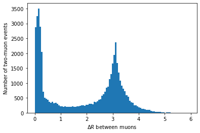
DeltaR
Another useful feature of these four-vector arrays is being able to compute deltaR (= sqrt(deltaEta^2 + deltaPhi^2)):
first_muon_p4.deltaR(second_muon_p4)plt.hist(first_muon_p4.deltaR(second_muon_p4), bins=100) plt.xlabel('$\Delta R$ between muons') plt.ylabel('Number of two-muon events') plt.show()
In principle, we could use this to clean up our invariant mass distribution, but we’ll skip that for simplicity.
Adding the four-vectors of the first muon and the second muon for all events is really as easy as:
sum_p4 = first_muon_p4 + second_muon_p4
sum_p4
<MomentumArray4D [{rho: 8.79, phi: 1.83, ... tau: 16.5}] type='48976 * Momentum4...'>
This is a 1D array of the four-vector sum for each event.
The last thing we need to do before we’re ready to plot the spectrum is to select only pairs with opposite charges:
two_muons_charges = branches['Muon_charge'][two_muons_mask]
opposite_sign_muons_mask = two_muons_charges[:, 0] != two_muons_charges[:, 1]
We apply this selection to the four-vector sums to get the dimuon four-vectors:
dimuon_p4 = sum_p4[opposite_sign_muons_mask]
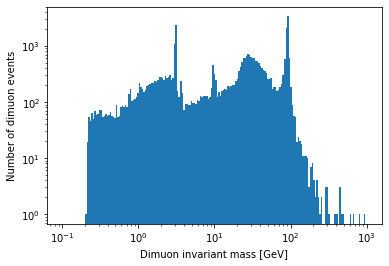
Exercise
Plot a histogram of the dimuon invariant mass on a log-log plot. Try to find all resonances (there are at least 7 visible). How many dimuon events are there?
Solution
plt.hist(dimuon_p4.mass, bins=np.logspace(np.log10(0.1), np.log10(1000), 200))
plt.xlabel('Dimuon invariant mass [GeV]')
plt.ylabel('Number of dimuon events')
plt.xscale('log')
plt.yscale('log')
plt.show()
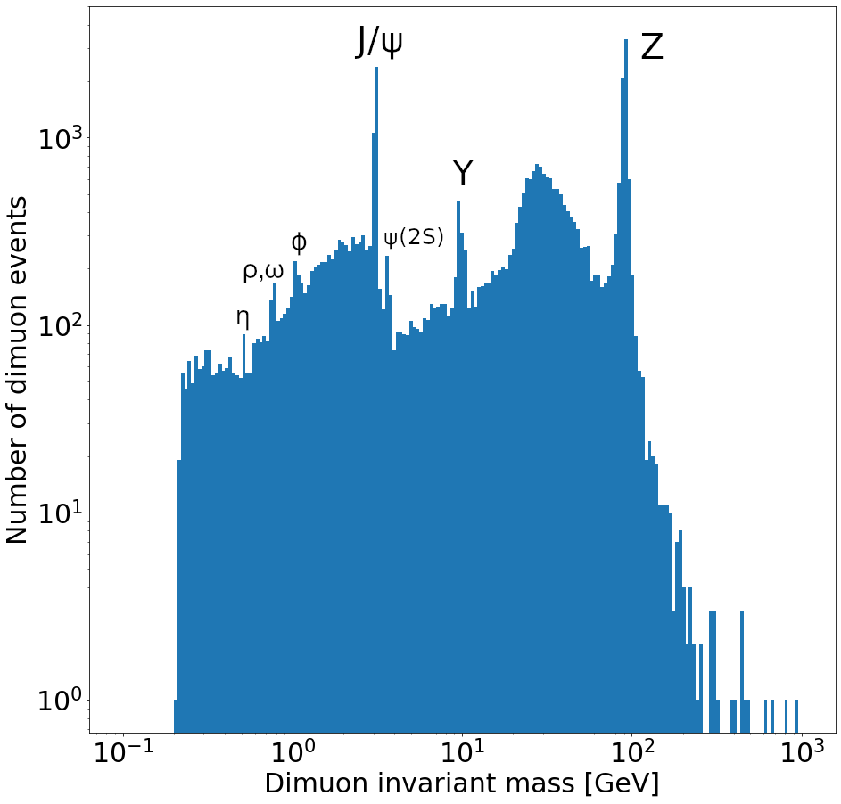
Labeled resonances:
len(dimuon_p4)37183
Key Points
Vector has allows you to manipulate arrays of four-vectors.
Uproot can be used to do real physics analyses.
Advanced topic: Fitting (optional)
Overview
Teaching: 0 min
Exercises: 0 minQuestions
How can I fit a common function to a histogram?
Objectives
Fit a distribution to the Z peak.
I want to zoom in on the Z resonance:
plt.hist(dimuon_p4.mass, bins=40, range=(70, 110))
plt.xlabel('Dimuon invariant mass [GeV]')
plt.ylabel('Number of dimuon events / 1 MeV')
plt.show()
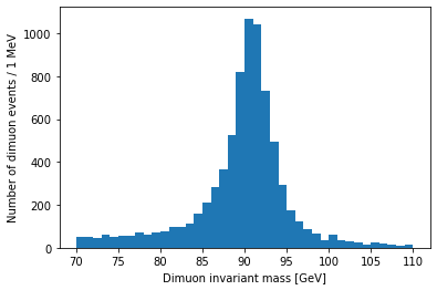
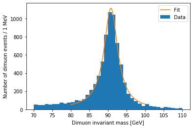
Resonances are described by the relativistic Breit-Wigner distribution. We should be able to fit one to this peak:
from scipy.optimize import curve_fit

def relativistic_breit_wigner(x, resonance_mass, width, normalization):
    gamma = np.sqrt(resonance_mass ** 2 * (resonance_mass ** 2 + width ** 2))
    k = 2.0 * np.sqrt(2) * resonance_mass * width * gamma / (np.pi * np.sqrt(resonance_mass ** 2 + gamma))
    return normalization * k / ((x ** 2 - resonance_mass ** 2) ** 2 + resonance_mass ** 2 * width ** 2)

bin_contents, bin_edges = np.histogram(dimuon_p4.mass.to_numpy(), bins=20, range=(80, 100))
bin_centers = (bin_edges[:-1] + bin_edges[1:]) / 2.0
popt, pcov = curve_fit(relativistic_breit_wigner, bin_centers, bin_contents, p0=[90, 10, 1000], sigma=np.sqrt(bin_contents))

plt.hist(dimuon_p4.mass, bins=40, range=(70, 110), label='Data')
x = np.linspace(80, 100, 200)
y = relativistic_breit_wigner(x, *popt)
plt.plot(x, y, label='Fit')
plt.xlabel('Dimuon invariant mass [GeV]')
plt.ylabel('Number of dimuon events / 1 MeV')
plt.legend()
plt.show()
.to_numpy()You may have noticed the
.to_numpy()used on the massArrayabove. As of Awkward Array 1.4.0, this is necessary fornp.histogram()to work, but this should be fixed in the next version.
The peak position is stored in popt[0]:
popt[0]
90.77360288470875
Pretty close to the real mass, 91.1876 GeV.
Key Points
There are many packages for fitting, and this just one very simple example.
Further resources
Overview
Teaching: 5 min
Exercises: 0 minQuestions
Where can I find more advanced information on these topics?
What other Python packages exist with tools for more complicated analysis?
Objectives
Find tutorials and documentation on Python tools (both generic and HEP-specific).
Caveat
One important note that I did not address at all: The methods that I showed here work great for operating on one small-ish file (smaller than your system’s RAM) at a time. Uproot has specialized methods and options that are better when running on many data files or larger files. This is one of many topics covered in the Uproot documentation below.
Scikit-HEP project
Uproot
Awkward Array
Vector
Other tools
Standard packages
- NumPy
- Matplotlib
- SciPy
- pandas (data frames)
Key Points
Python and many Python packages have a huge userbase and are well supported by documentation, tutorials, and the community.