Columnar Analysis
Overview
Teaching: 25 min
Exercises: 5 minQuestions
What is columnar analysis?
What are its advantages over row-based analysis?
How do I perform selections and operations on columns?
Objectives
Count items passing some selection criteria.
Apply selection criteria to get passing events/objects.
Plot different selections for comparison.
Uproot is designed for columnar analysis, which means performing operations on entire columns (branches) at a time, rather than operating on every event individually.
Counting
The simplest task we need for analysis is counting (i.e., cutflow).
To count the total number of events, we can use the Python built-in function len() on any of the following:
len(branches)
len(branches['nMuon'])
len(branches['Muon_pt']) # or any of the other branches...
100000
So there are 100,000 events.
Exercise
Note that this is not the total number of muons, despite running
len()on a branch that has a number for every single muon (Muon_pt)! Why is this? Can you write some code that does give the total number of muons in the file?Solution
len()only looks at the length along the first dimension of the array.Muon_ptis a 2D array. In order to count every muon individually, we need to flatten the array to 1D.len(ak.flatten(branches['Muon_pt']))235286
Selections
Selections from 1D arrays
To do more interesting counting or plotting, we want to be able to select only events or muons that pass some criteria.
Just as you can compare two numbers, like 1 < 2 and get a True or False value, you can put arrays in comparisons as well.
Let’s look at this case:
branches['nMuon'] == 1
<Array [False, False, True, ... False, False] type='100000 * bool'>
This is checking for equality between an array and the number 1.
Of course these are different types (array vs. scalar), so the Python objects are certainly not identical, but you can see the return value is not just False.
What happens is that each element in the array is compared to the scalar value, and the return value is a new array (of the same shape) filled with all these comparison results.
So we can interpret the output as the result of testing whether each event has exactly one muon or not.
The first two events do not, the third does, and so on.
This array of Boolean values is called a mask because we can use it to pick out only the elements in the array that satisfy some criteria (like having exactly one muon). This is very useful, and we will save it to a variable to save typing later:
single_muon_mask = branches['nMuon'] == 1
Counting with selections
Now let’s say we want to know how many of these single-muon events there are.
Note that len() won’t work because the length of the array is still 100,000.
That is, there’s a value for every event (even if that value is False).
We need the number of Trues in the array.
There are multiple ways to do this, but my favorite is:
np.sum(single_muon_mask)
13447
sum() adds all the array values together.
True is interpreted as 1 and False is interpreted as 0, thus sum() is just the number of True entries.
So there are 13,447 events with exactly one muon.
Applying a mask to an array
If we want to apply some selection to an array (i.e., cut out events or muons that don’t pass), we just act like the selection mask is an index. For example, if we want the pT of only those muons in events with exactly one muon (so they’re the only muon in that event):
branches['Muon_pt'][single_muon_mask]
<Array [[3.28], [3.84], ... [13.3], [9.48]] type='13447 * var * float32'>
We can check that we really are only looking at the events that pass the selection by looking the number of rows:
len(branches['Muon_pt'][single_muon_mask])
13447
Yep, this matches the counting from single_muon_mask.sum() above.
Plotting with selections
We can also use masks to plot quantities after some selection. For example, let’s plot the muon pT for only the single-muon events:
plt.hist(ak.flatten(branches['Muon_pt'][single_muon_mask]), bins=100, range=(0, 100))
plt.xlabel('Muon $p_{\mathrm{T}}$ [GeV]')
plt.ylabel('Number of single muons / 1 GeV')
plt.yscale('log')
plt.show()
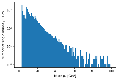
If you’re looking carefully, you might notice that this plot is missing the hump around 45 GeV that was in the pT plot before (for all muons). We accidentally ran into a hint of an effect from real physics. Neat!
Selections from a jagged array
Let’s look at a comparison for a jagged array, using the absolute value of muon eta:
eta_mask = abs(branches['Muon_eta']) < 2
eta_mask
<Array [[True, True], ... True, True, True]] type='100000 * var * bool'>
Again, the mask array has the same dimensions as the original array. There’s one Boolean value for each muon, corresponding to whether its eta is less than 2 in absolute value.
Counting
We can do counting and plotting just as before:
np.sum(eta_mask)
204564
This is the number of muons that pass the eta cut.
Plotting
Let’s plot both the original eta distribution and the one after the cut to verify its effect:
plt.hist(ak.flatten(branches['Muon_eta']), bins=50, range=(-2.5, 2.5))
plt.title('No selection')
plt.xlabel('Muon $\eta$')
plt.ylabel('Number of muons')
plt.show()

plt.hist(ak.flatten(branches['Muon_eta'][eta_mask]), bins=50, range=(-2.5, 2.5))
plt.title('With $|\eta| < 2$ selection')
plt.xlabel('Muon $\eta$')
plt.ylabel('Number of muons')
plt.show()
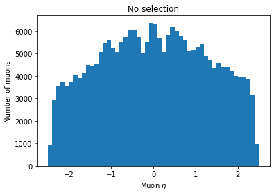
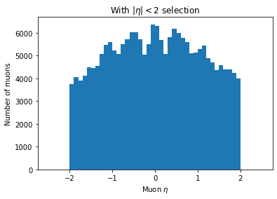
You can see the second plot just has both ends past 2 cut off, demonstrating that we’ve cut those muons out.
Operations on selections
We can invert selections with ~ (the NOT operator):
~single_muon_mask
<Array [True, True, False, ... True, True] type='100000 * bool'>
This new mask is False only for events with exactly one muon and True otherwise.
We can get the intersection of selections with & (the AND operator):
single_muon_mask & eta_mask
<Array [[False, False], ... False, False]] type='100000 * var * bool'>
This mask is True only for muons with no other muons in their event and abs(eta) < 2.
Or we can get the union of selections with | (the OR operator):
single_muon_mask | eta_mask
<Array [[True, True], ... True, True, True]] type='100000 * var * bool'>
This mask is True for muons which are the only muon in their event or which have abs(eta) < 2.
Warning about combining selections
You have to be careful about combining comparisons with the operators above. Consider the following expression:
False == False & FalseTrueIt’s a common mistake to assume that this expression would be
Falseby interpreting it as:(False == False) & FalseFalseThe issue is that
&has a higher precedence than==, so the first expression is actually equivalent to:False == (False & False)TrueWhat this means is that parentheses are necessary for expressions like this to have the correct meaning:
(branches['nMuon'] == 1) & (abs(branches['Muon_eta']) < 2)
Comparing histograms
Now we can use these operations to compare distributions for different selections.
Let’s look at the pT of single-event muons split into two groups by whether or not abs(eta) < 2.
All we have to do is provide a list of arrays as the first argument to hist rather than just one array.
Note the square brackets around the two arrays:
plt.hist([ak.flatten(branches['Muon_pt'][single_muon_mask & eta_mask]),
          ak.flatten(branches['Muon_pt'][single_muon_mask & ~eta_mask])],
         bins=25, range=(0, 50))
plt.xlabel('Muon $p_{\mathrm{T}}$ [GeV]')
plt.ylabel('Number of single muons / 2 GeV')
plt.show()
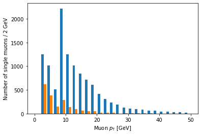
Ah, but it doesn’t actually say which histogram is which. For that, we need to add labels and a legend:
plt.hist([ak.flatten(branches['Muon_pt'][single_muon_mask & eta_mask]),
          ak.flatten(branches['Muon_pt'][single_muon_mask & ~eta_mask])],
         label=['$|\eta| < 2$', '$|\eta| \geq 2$'],
         bins=25, range=(0, 50))
plt.xlabel('Muon $p_{\mathrm{T}}$ [GeV]')
plt.ylabel('Number of single muons / 2 GeV')
plt.legend()
plt.show()
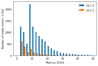
label is a list of strings passed to hist, corresponding to the arrays (in the same order),
and we have to add plt.legend() in order to actually draw a legend with those labels.
Another problem is that these histograms are on different scales because there are fewer large eta muons.
Often we want to compare only the shapes of the distribution, so we normalize the integral of each to 1.
We can achieve this by adding density=True to the hist() call:
plt.hist([ak.flatten(branches['Muon_pt'][single_muon_mask & eta_mask]),
          ak.flatten(branches['Muon_pt'][single_muon_mask & ~eta_mask])],
         label=['$|\eta| < 2$', '$|\eta| \geq 2$'],
         bins=25, range=(0, 50), density=True)
plt.title('Normalized')
plt.xlabel('Muon $p_{\mathrm{T}}$ [GeV]')
plt.ylabel('Number of single muons / 2 GeV')
plt.legend()
plt.show()
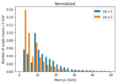
Now we can clearly see there’s a significantly higher fraction of muons with abs(eta) >= 2 at lower pT compared to muons with abs(eta) < 2. This makes geometric sense, since muons at higher abs(eta) are traveling in a direction less perpendicular to the beam.
(This name of the density parameter refers to the idea of interpreting the histogram as a probability density function, which always has an integral of 1.)
Columnar vs. row-based analysis
As an aside about columnar analysis, take a look at this comparison of speed for counting muons with abs(eta) < 2.
The first example is a row-based approach, using
forloops over every event and every muon in the event:%%time eta_count = 0 for event in branches['Muon_eta']: for eta in event: if abs(eta) < 2: eta_count += 1 eta_countCPU times: user 4.78 s, sys: 77.2 ms, total: 4.86 s Wall time: 4.88 s 204564The next example uses columnar operations, running on all muons at once:
%%time

np.sum(abs(branches['Muon_eta']) < 2)
CPU times: user 5.18 ms, sys: 1 ms, total: 6.18 ms Wall time: 4.87 ms 204564The columnar approach here is about 1000 times faster.
Key Points
Selections are created by comparisons on arrays and are represented by masks (arrays of Boolean values).
Selections are applied by acting like a mask is an array index.
Avoid
forloops whenever possible in analysis (especially in Python).