Introduction

Overview

Teaching: 15 min
Exercises: 0 min

Questions

What is machine learning?

What role does machine learning have in high energy physics?

What should I do if I want to get good at machine learning?

Objectives

Discuss the general learning task in machine learning.

Provide examples of machine learning in high energy physics.

Give resources to people who want to become proficient in machine learning.

What is Machine Learning?

General definition

-Arthur Samuel, 1959

In a traditional approach to solving problems, one would study a problem, write rules (i.e. laws of physics) to solve that problem, analyze errors, then modify the rules. A machine learning approach automates this process: a machine learning model modifies its rules based on the errors it measures. This abstract statement becomes more conceptual once the mathematical foundations are established. For now, you can think of the following example:

One wishes to fit some data points to a best fit line $y=ax+b$. One chooses initial “guesses” for $a$ and $b$ and a machine learning algorithm finds the optimal values of $a$ and $b$ with respect to the mean-squared error.

There are three main tasks in machine learning:

Regression. The input is multi-dimensional data points and the output is a real number (or sequence of real numbers). For example, the input might be height and weight, whilst output might be resting heart rate and resting blood pressure (a sequence of real numbers).
Classification. The input is multi-dimensional data points and the output is an integer (which represents different classes). Consider the following example with two classes: pictures of roses and pictures of begonias. The input would be multi-dimensional images (color channel included) and one may assign the integer 0 to roses and the integer 1 to begonias.
Generation: The input is noise and the output is something sensible. For example, training a machine learning algorithm to take in a random seed and generate images of peoples faces. Another example could be ageing filters on social media.

What Role Does Machine Learning have in High Energy Physics?

One may want to classify detected particles as signal or background events based on their energy, momentum, charge, etc… . This specific problem was featured on Kaggle in 2014 here. This problem will also be examined in this tutorial.
(My research) I want to make measurements of a rare signal process. Background processes that look similar to the rare signal process are much more common. A machine learning technique can optimise at the same time the use of many variables that separate signal and background. Not only does a machine learning technique optimise the use of many variables at the same time, but it can find correlations in many dimensions that will give better signal/background classification than individual variables ever could. This is an example of classification in action. Again, this is similar to what we’ll be exploring in this tutorial!

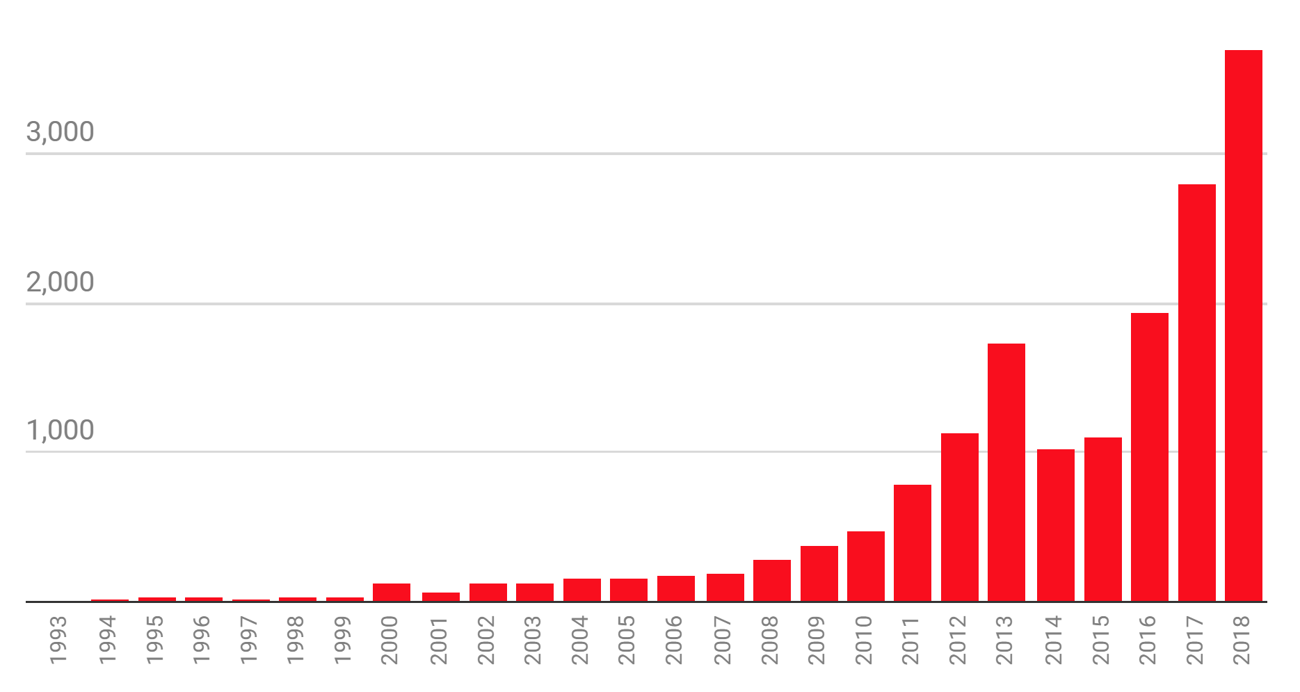
Machine learning has become quite popular in scientific fields in the past few years. The following plot from MIT Technical Review examines the number of papers available in the “artificial intelligence” section of arXiv up to November 18, 2018.

ML Popularity

The following are a few recent articles on machine learning in high energy physics

Where to Become Proficient in Machine Learning

Machine Learning is not something you’ll learn in an hour. It’s a skill you need to develop over time, and like any skill you need to practice a little bit every day. If you want to really excel at machine learning, my recommendation is to try an online course such as this one. If textbooks are your thing, try this book, ensuring to read and code along with each chapter. Don’t go crazy: just do 30 minutes a day. You’d be surprised how much you could learn in a couple months. In summary:

For Learning Essential Python libraries: this online article for an introduction or this textbook if you have it available
For Learning Machine Learning libraries: this online article for an introduction or this textbook if you have it available

Just for a bit of perspective, I started learning about machine learning in April 2019. Don’t expect the learning process to be a quick one: follow online courses and code along with them. If you have a textbook, read through it thoroughly and make sure you code along with the textbook.

Your feedback is very welcome! Most helpful for us is if you “Improve this page on GitHub”. If you prefer anonymous feedback, please fill this form.

Key Points

The 3 main tasks of Machine Learning are regression, classification and generation.

Machine learning has many applications in high energy physics.

If you want to become proficient in machine learning, you need to practice.

Mathematical Foundations

Overview

Teaching: 20 min
Exercises: 0 min

Questions

What is the common terminology in machine learning?

How does machine learning actually optimize?

Is there anything I should be careful of?

Objectives

Discuss the role of data, models, and loss functions in machine learning.

Discuss the role of gradient descent when optimizing a model.

Alert you to the dangers of overfitting!

In this section we will establish the mathematical foundations of machine learning. We will define three important quantities: data, models, and loss functions. We will then discuss the optimization procedure known as gradient descent.

Definitions

Some common definitions are included below.

Data $(x_i, y_i)$ where $i$ represents the $i^{\text{th}}$ data point. The $x_i$ are typically referred to as instances and the $y_i$ as labels. In general the $x_i$ and $y_i$ don’t need to be numbers. For example, in a dataset consisting of pictures of animals, the $x_i$ might be images (consisting of height, width, and color channel) and the $y_i$ might be a string which states the type of animal.
Model: Some abstract function $f$ such that $y=f(x;\theta)$ is used to model the individual $(x_i, y_i)$ pairs. $\theta$ is used to represent all necessary parameters in the function, so it can be thought of as a vector. For example, if the $(x_i, y_i)$ are real numbers and approximately related through a quadratic function, then an adequate model might be $f(x;a,b,c)=ax^2+bx+c$. Note that one could also use the model $f(x;a,b,c,...)=ax^3+b\sin(x)+ce^x + ...$ to model the dataset; a model is just some function; it doesn’t need to model the data well necessarily. For the case where the $x_i$ are pictures of animals and the $y_i$ are strings of animal names, the function $f$ may need to be quite complex to achieve reasonable accuracy.
Loss Function: A function that determines how well the model $y=f(x)$ predicts the data $(x_i, y_i)$. Some models work better than others. One such loss function might be $\sum_i (y_i-f(x_i))^2$: the mean-squared error. For the quadratic function this would be $\sum_i (y_i-(ax_i^2+bx_i+c))^2$. One doesn’t need to use the mean-squared error (MSE) as a loss function, however; one could also use the mean-absolute error (MAE), or the mean-cubed error, etc. What about cases where the $x_i$ represent pictures of animals and the $y_i$ are strings representing the animal in the picture? How can we define a loss function to account for the error the function made when classifying this picture? In this case one needs to be clever about loss functions as functions like the MSE or MAE don’t make sense anymore. A common loss function in this case is the cross entropy loss function.

Loss Function and Likelihood

Likelihood measures the goodness of fit of a statistical model to a data sample. For computational convenience, the log-likelihood is often used Wikipedia. The MSE loss function is a special case of using the maximum log-likelihood method when the model $f$ describes measurements as outcomes of independent Gaussian random variables where each random variable has the same standard deviation. In this case $\ln \mathcal{L}(\theta) = \text{const.} - \frac{1}{2\sigma^2} \sum_{i=1}^N (y_i-f(x_i, \theta))^2$ where $\mathcal{L}$ is the likelihood function, $(x_i, y_i)$ are the data, $\sigma$ is the standard deviation of the random variables, and $\theta$ represents the model parameters. Since we subtract the loss function in the formula for log-likelihood, minimizing the MSE loss function is equivalent to maximizing the likelihood.

Quadratic model and data points

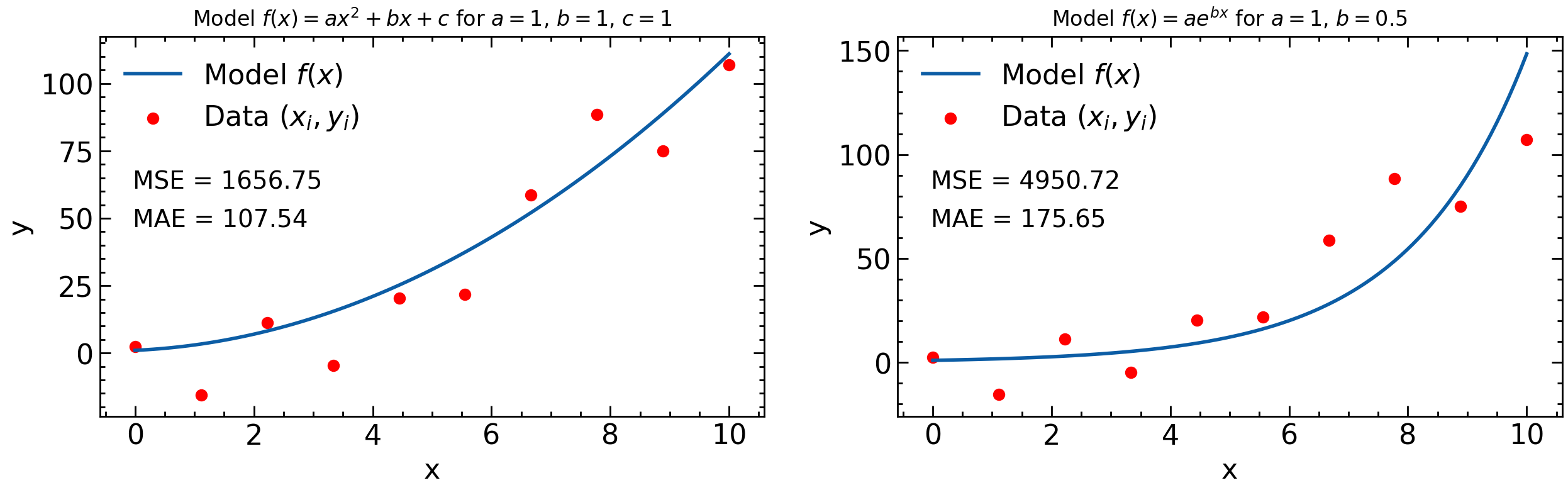
What’s important to note is that once the data and model are specified, then the loss function depends on the parameters of the model. For example, consider the data points $(x_i, y_i)$ in the plot above and the MSE loss function. For the left hand plot the model is $y=ax^2+bx+c$ and so the MSE depends on $a$, $b$, and $c$ and the loss function, $L=L(\theta)=L(a,b,c)$. For the right hand plot, however, the model is $y=ae^{bx}$ and so in this case the MSE only depends on two parameters: $a$ and $b$ and $L(\theta)=L(a,b)$.

Gradient Descent

For most applications, the goal of machine learning is to optimize a loss function with respect to the parameters of a model given a dataset and a model. Lets suppose we have the dataset $(x_i, y_i)$, the model $y=ax^2+bx+c$, and we use the loss function $L(\theta) = L(a, b, c) = \sum_i (y_i-(ax_i^2+bx_i+c))^2$ to determine the validity of the model. We want to minimize the loss function with respect to $a$, $b$, and $c$ (thus creating the best model). One such way to do this is to pick some random initial values for $a$, $b$, and $c$, and then repeat the following two steps until we reach a minimum for $L(a,b,c)$

Evaluate the gradient $\nabla_{\theta} L$. The negative gradients points to where the function $L(\theta)$ is decreasing.
Update $\theta \to \theta - \alpha \nabla_{\theta} L$ The parameter $\alpha$ is known as the learning rate in machine learning.

This procedure is known as gradient descent in machine learning. It’s sort of like being on a mountain, and only looking at your feet to try and reach the bottom. You’ll likely move in the direction where the slope is decreasing the fastest. The problem with this technique is that it may lead you into local minima (places where the mountain has “pits” but you’re not at the base of the mountain).

Quadratic model and data points

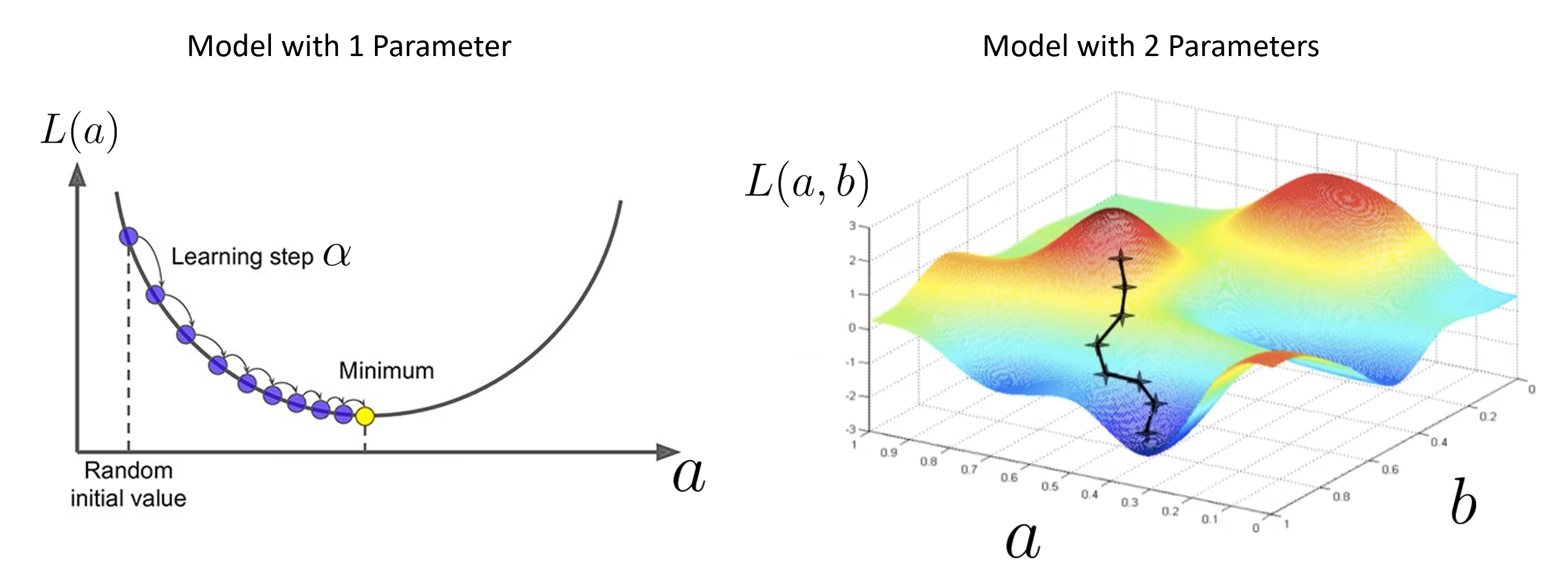
Note that the models in the plots above have 1 (left) and 2 (right) parameters. A typical neural network can have $O(10^4)$ parameters. In such a situation, the gradient is a vector with dimensions $O(10^4)$; this can be computationally expensive to compute. In addition, the gradient $\nabla_{\theta} L$ depends on all the data points $(x_i, y_i)$. This is often computationally expensive for datasets that include many data points. Typical machine learning data sets can have millions of (multi-dimesional) data points. A solution to this is to sample a different small subset of points each time the gradient is computed. This is known as batch gradient descent.

The Fly in the Ointment: Overfitting

Quadratic model and data points

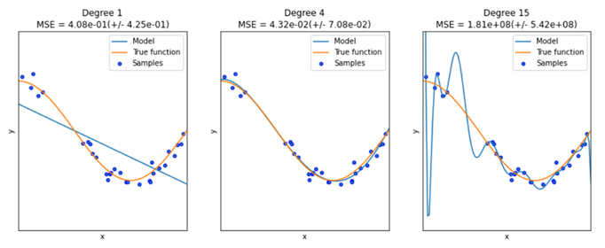
In general, a model with more parameters can fit a more complicated dataset. Consider the plot above for a case where we happen to know the true function

A model with too few parameters (left) can’t describe the data (underfitting)
A model with too many parameters (right) will learn the statistical fluctuations in the data and doesn’t describe the general trend well (overfitting)
You’re aiming for the goldilocks number of parameters in the middle!

In general you want to train the model on some known data points $(x_i,y_i)$ and then use the model to make predictions on new data points, but if the model is overfitting then the predictions for the new data points will be inaccurate.

The main way to avoid the phenomenon of overfitting in machine learning is by using what is known as a training set $(x_i, y_i)_t$ and a validation set $(x_i, y_i)_v$. The training set typically consists of 60%-80% of your data and the validation set consists of the rest of the data. During training, one only uses the the training set to tune $\theta$. One can then determine if the model is overfitting by comparing $L(\theta)$ for the training set and the validation set. Typically, the model will start to overfit after a certain number of gradient descent steps: a straightforward way to stop overfitting is to stop adjusting $\theta$ using gradient descent when the loss function starts to significantly differ between training and validation.

Regression, Classification, Generation

The three main tasks of machine learning can now be revisited with the mathematical formulation.

Regression. The data in this case are $(x_i, y_i)$, where the $y_i$ are continuous in $\mathbb{R}^n$. For example, each instance $x_i$ might specify the height and weight of a person and $y_i$ the corresponding resting heart rate of the person. A common loss function for this type of problem is the MSE.
Classification. The data in this case are $(x_i, y_i)$, where $y_i$ are discrete values that represent classes. For example, each instance $x_i$ might specify the petal width and height of a flower and each $y_i$ would then specify the corresponding type of flower. A common loss function for this type of problem is cross entropy. In these learning tasks, a machine learning model typically predicts the probability that a given $x_i$ corresponds to a certain class. Hence if the possible classes in the problem are $(C_1, C_2, C_3, C_4)$ then the model would output an array $(p_1, p_2, p_3, p_4)$ where $\sum_i p_i = 1$ for each $y_i$.
Generation. As discussed previously, the input is a random distribution (typically Gaussian noise) and the output is some data: typically an image. You can think of the input as codings of the image to be generated. This process is fundamentally different than regression or classification. For more information see Wikipedia for an introduction or if you have it available, Chapter 17 of Hands-On Machine Learning where Generative Adversarial Networks are discussed.

Your feedback is very welcome! Most helpful for us is if you “Improve this page on GitHub”. If you prefer anonymous feedback, please fill this form.

Key Points

In a particular machine learning problem, one needs an adequate dataset, a reasonable model, and a corresponding loss function. The choice of model and loss function needs to depend on the dataset.

Gradient descent is a procedure used to optimize a loss function corresponding to a specific model and dataset.

Beware of overfitting!

Neural Networks

Overview

Teaching: 10 min
Exercises: 10 min

Questions

What is a neural network?

How can I visualize a neural network?

Objectives

Examine the structure of a fully connected sequential neural network.

Look at the TensorFlow neural network Playground to visualize how a neural network works.

Neural Network Theory Introduction

Here we will introduce the mathematics of a neural network. You are likely familiar with the linear transform $y=Ax+b$ where $A$ is a matrix (not necessarily square) and $y$ and $b$ have the same dimensions and $x$ may have a different dimension. For example, if $x$ has dimension $n$ and $y$ and $b$ have dimensions $m$ then the matrix $A$ has dimension $m$ by $n$.

Now suppose we have some vector $x_i$ listing some features (height, weight, body fat) and $y_i$ contains blood pressure and resting heart rate. A simple linear model to predict the label features given the input features is then $y=Ax+b$ or $f(x)=Ax+b$. But we can go further. Suppose we also apply a simple but non-linear function $g$ to the output so that $f(x) = g(Ax+b)$. This function $g$ does not change the dimension of $Ax+b$ as it is an element-wise operation. This function $g$ is known as an activation function. The activation function defines the output given an input or set of inputs. The purpose of the activation function is to introduce non-linearity into the output (Wikipedia). Non-linearity allows us to describe patterns in data that are more complicated than a straight line. A few activation functions $g$ are shown below.

Quadratic model and data points

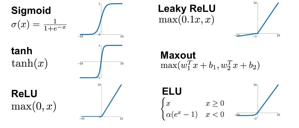
(No general picture is shown for the Maxout function since it depends on the number of w and b used)

Each of these 6 activation functions has different advantages and disadvantages.

Now we can perform a sequence of operations to construct a highly non-linear function. For example; we can construct the following model:

[f(x) = g_2(A_2(g_1(A_1x+b_1))+b_2)]

We first perform a linear transformation, then apply activation function $g_1$, then perform another linear transformation, then apply activation function $g_2$. The input $x$ and the output $f(x)$ are not necessarily the same dimension.

For example, suppose we have an image (which we flatten into a 1d array). This array might be 40000 elements long. If the matrix $A_1$ has 2000 rows, we can perform one iteration of $g_1(A_1x+b_1)$ to reduce this to a size of 2000. We can apply this over and over again until eventually only a single value is output. This is the foundation of a fully connected neural network. Note we can also increase the dimensions throughout the process, as seen in the image below. We start with a vector $x$ of size 3, perform the transformation $g_1(A_1x+b_1)$ so the vector is size 4, then perform one final transformation so the vector is size 2.

Quadratic model and data points

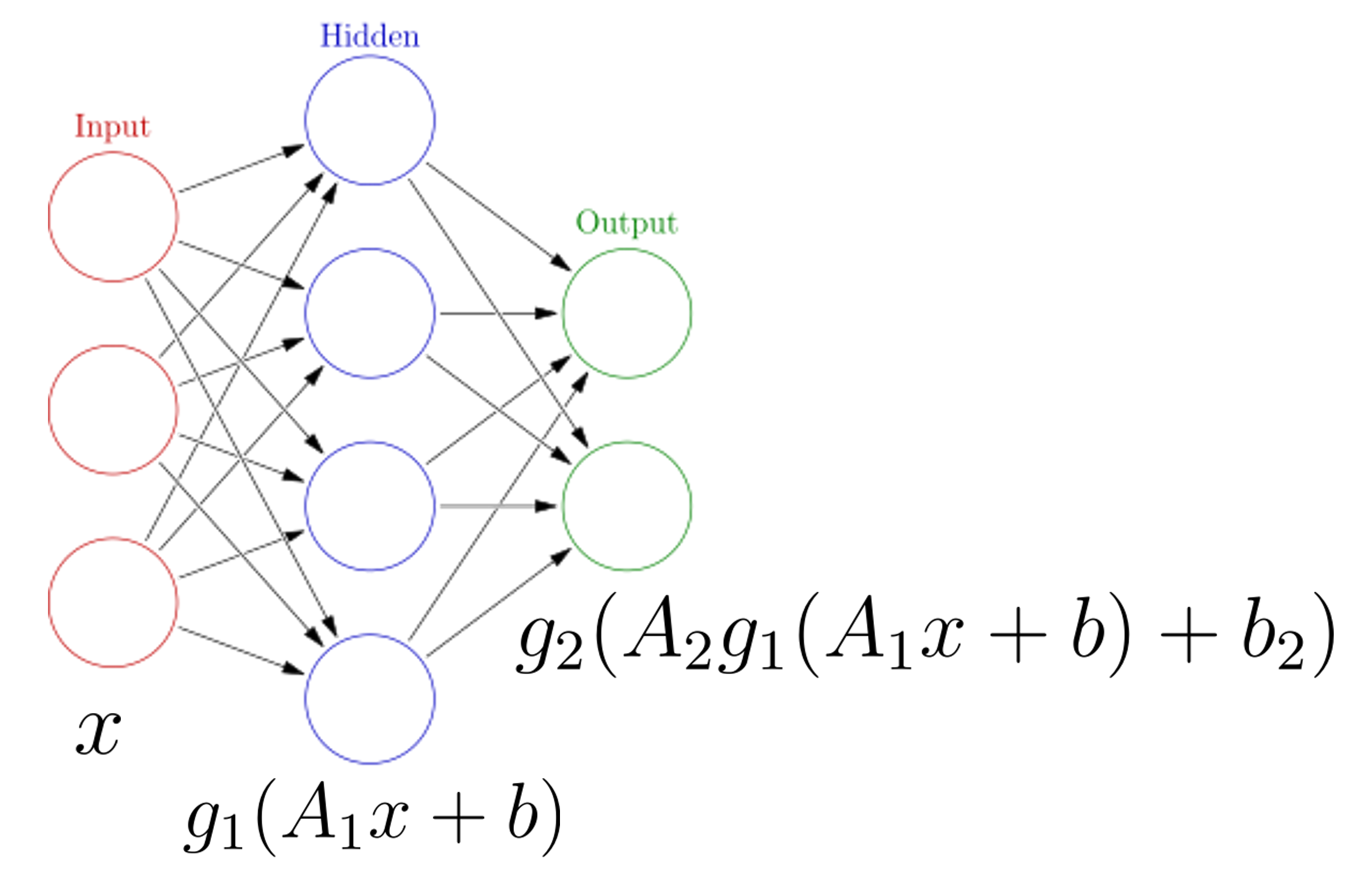
The vector $x$ is referred to as the input layer of the network
Intermediate quantities (such as $g_1(A_1x+b_1)$) are referred to as hidden layers. Each element of the vector $g_1(A_1x+b_1)$ is referred to as a neuron.
The model output $f(x)$ is referred to as the output layer. Note that activation functions are generally not used in the output layer.

Neural networks require a careful training procedure. Suppose we are performing a regression task (for example we are given temperature, wind speed, wind direction and pressure, and asked to predict relative humidity). The final output of the neural network will be a single value. During training, we compare the outputs of the neural network $f(x_i)$ to the true values of the data $y_i$ using some loss function $L$. We need to tune the parameters of the model so that $L$ is as small as possible. What are the parameters of the model in this case? The parameters are the elements of the matrices $A_1, A_2, ...$ and the vectors $b_1, b_2, ...$. We also need to adjust them in an appropriate fashion so we are moving closer to the minimum of $L$. For this we need to compute $\nabla L$. Using a clever technique known as back-propagation, we can determine exactly how much each parameter (i.e. each entry in matrix $A_i$) contributes to $\nabla L$. Then we slightly adjust each parameter such that $\vec{L} \to \vec{L}-\alpha \nabla{L}$ where, as before, $\alpha$ is the learning rate. Through this iterative procedure, we slowly minimize the loss function.

TensorFlow Playground

See here for an interactive example of a neural network structure. Why not play around for about 10 minutes!

Your feedback is very welcome! Most helpful for us is if you “Improve this page on GitHub”. If you prefer anonymous feedback, please fill this form.

Key Points

Neural networks consist of an input layer, hidden layers and an output layer.

TensorFlow Playground is a cool place to visualize neural networks!

Comfort break!

Overview

Teaching: 0 min
Exercises: 15 min

Questions

Get up, stretch out, take a short break.

Objectives

Refresh your mind.

Key Points

You’ll be back.

They’re the jedi of the sea.

Resources

Overview

Teaching: 10 min
Exercises: 0 min

Questions

Where should I go if I want to get better at Python?

What are the machine learning libraries in Python?

Objectives

Provide links to tutorials and textbooks that will help you get better at Python.

Provide links to machine learning library documentation.

Proficiency in Python

If you are unfamiliar with Python, the following tutorials will be useful:

For non-trivial machine learning tasks that occur in research, one needs to be proficient in the programming libraries discussed in the tutorial here. There are two main python libraries for scientific computing:

NumPy: the go-to numerical library in Python. See the documentation. NumPy’s main purpose is the manipulation of multi-dimensional arrays: this includes both
- slicing: taking “chunks” out of arrays. Slicing in Python means taking elements from one given index to another given index. For 1 dimensional arrays this reduces to selecting intervals, but these operations can become quite advanced for multidimesional arrays.
- functional operations: applying a function to an entire array. This code is highly optimized: there is often a myth that Python is slower than languages like C++; while this may be true for things like for-loops, it is not true if you use NumPy properly.
pandas: pandas is a fast, powerful, flexible and easy to use open source data analysis and manipulation tool, built on top of the Python programming language. See the documentation. The most important datatype in the pandas library is the DataFrame: a “spreadsheet-type object” with row and column names. It is preferred to use pandas DataFrames rather than NumPy arrays for managing data sets.

If you are unfamiliar with these packages, I would recommend reading the introduction to the documentation pages for NumPy slicing, NumPy operations and pandas DataFrames or sitting down with this textbook if you have it available and reading/coding along with chapters 4 and 5. In a few hours, you should have a good idea of how these packages work.

Machine Learning Libraries in Python

There are many machine libraries in Python, but the two discussed in this tutorial are scikit-learn and PyTorch.

scikit-learn: features various classification, regression and clustering algorithms and is designed to interoperate with the Python numerical and scientific libraries NumPy and SciPy. See the documentation.
PyTorch: PyTorch is an end-to-end open-source platform for machine learning. It is used for building and deploying machine learning models. See the documentation.

What about GPUs?

scikit-learn doesn’t have GPU support, therefore should only be used for training simple neural networks.

PyTorch does have GPU support, therefore can be used to train complicated neural network models that require a lot of GPU power.

Take a look at our tutorial “Machine Learning on GPUs” if you’re interested.

Note that the four Python programming packages discussed so far are interoperable: in particular, datatypes from NumPy and pandas are often used in packages like scikit-learn and PyTorch.

Your feedback is very welcome! Most helpful for us is if you “Improve this page on GitHub”. If you prefer anonymous feedback, please fill this form.

Key Points

NumPy and pandas are the main libraries for scientific computing.

scikit-learn and PyTorch are two good options for machine learning in Python.

Data Discussion

Overview

Teaching: 10 min
Exercises: 5 min

Questions

What dataset is being used?

How do some of the variables look?

Objectives

Briefly describe the dataset.

Take a peek at some variables.

Code Example

Here we will import all the required libraries for the rest of the tutorial. All scikit-learn and PyTorch functions will be imported later on when they are required.

import pandas as pd  # to store data as dataframe
import numpy as np  # for numerical calculations such as histogramming
import matplotlib.pyplot as plt  # for plotting

You can check the version of these packages by checking the __version__ attribute.

np.__version__

Let’s set the random seed that we’ll be using. This reduces the randomness when you re-run the notebook

seed_value = 420  # 42 is the answer to life, the universe and everything
from numpy.random import seed  # import the function to set the random seed in NumPy

seed(seed_value)  # set the seed value for random numbers in NumPy

Dataset Used

The dataset we will use in this tutorial is simulated ATLAS data. Each event corresponds to 4 detected leptons: some events correspond to a Higgs Boson decay (signal) and others do not (background). Various physical quantities such as lepton charge and transverse momentum are recorded for each event. The analysis in this tutorial loosely follows the discovery of the Higgs Boson.

# In this notebook we only process the main signal ggH125_ZZ4lep and the main background llll,
# for illustration purposes.
# You can add other backgrounds after if you wish.
samples = ["llll", "ggH125_ZZ4lep"]

Exploring the Dataset

Here we will format the dataset $(x_i, y_i)$ so we can explore! First, we need to open our data set and read it into pandas DataFrames.

# get data from files

DataFrames = {}  # define empty dictionary to hold dataframes
for s in samples:  # loop over samples
    DataFrames[s] = pd.read_csv("/kaggle/input/4lepton/" + s + ".csv")  # read .csv file

DataFrames["ggH125_ZZ4lep"]  # print signal data to take a look

Before diving into machine learning, think about whether there are any things you should do to clean up your data. In the case of this Higgs analysis, Higgs boson decays should produce 4 electrons or 4 muons or 2 electrons and 2 muons. Let’s define a function to keep only events which produce 4 electrons or 4 muons or 2 electrons and 2 muons.

# cut on lepton type
def cut_lep_type(lep_type_0, lep_type_1, lep_type_2, lep_type_3):
    # first lepton is [0], 2nd lepton is [1] etc
    # for an electron lep_type is 11
    # for a muon lep_type is 13
    # only want to keep events where one of eeee, mumumumu, eemumu
    sum_lep_type = lep_type_0 + lep_type_1 + lep_type_2 + lep_type_3
    if sum_lep_type == 44 or sum_lep_type == 48 or sum_lep_type == 52:
        return True
    else:
        return False

We then need to apply this function on our DataFrames.

# apply cut on lepton type
for s in samples:
    # cut on lepton type using the function cut_lep_type defined above
    DataFrames[s] = DataFrames[s][
        np.vectorize(cut_lep_type)(
            DataFrames[s].lep_type_0,
            DataFrames[s].lep_type_1,
            DataFrames[s].lep_type_2,
            DataFrames[s].lep_type_3,
        )
    ]
DataFrames["ggH125_ZZ4lep"]  # print signal data to take a look

Challenge

Another cut to clean our data is to keep only events where lep_charge_0+lep_charge_1+lep_charge_2+lep_charge_3==0. Write out this function yourself then apply it.

Solution

# cut on lepton charge
def cut_lep_charge(lep_charge_0,lep_charge_1,lep_charge_2,lep_charge_3):
# only want to keep events where sum of lepton charges is 0
    sum_lep_charge = lep_charge_0 + lep_charge_1 + lep_charge_2 + lep_charge_3
    if sum_lep_charge==0: return True
    else: return False

# apply cut on lepton charge
for s in samples:
    # cut on lepton charge using the function cut_lep_charge defined above
    DataFrames[s] = DataFrames[s][ np.vectorize(cut_lep_charge)(DataFrames[s].lep_charge_0,
                                                    	    DataFrames[s].lep_charge_1,
                                                    	    DataFrames[s].lep_charge_2,
                                                    	    DataFrames[s].lep_charge_3) ]
DataFrames['ggH125_ZZ4lep'] # print signal data to take a look

Plot some input variables

In any analysis searching for signal one wants to optimise the use of various input variables. Often, this optimisation will be to find the best signal to background ratio. Here we define histograms for the variables that we’ll look to optimise.

lep_pt_2 = {  # dictionary containing plotting parameters for the lep_pt_2 histogram
    # change plotting parameters
    "bin_width": 1,  # width of each histogram bin
    "num_bins": 13,  # number of histogram bins
    "xrange_min": 7,  # minimum on x-axis
    "xlabel": r"$lep\_pt$[2] [GeV]",  # x-axis label
}

Challenge

Write a dictionary of plotting parameters for lep_pt_1, using 28 bins. We’re using 28 bins here since lep_pt_1 extends to higher values than lep_pt_2.
Solution
lep_pt_1 = { # dictionary containing plotting parameters for the lep_pt_1 histogram
    # change plotting parameters
    'bin_width':1, # width of each histogram bin
    'num_bins':28, # number of histogram bins
    'xrange_min':7, # minimum on x-axis
    'xlabel':r'$lep\_pt$[1] [GeV]', # x-axis label
}

Now we define a dictionary for the histograms we want to plot.

SoverB_hist_dict = {
    "lep_pt_2": lep_pt_2,
    "lep_pt_1": lep_pt_1,
}  # add a histogram here if you want it plotted

Now let’s take a look at those variables. Because the code is a bit long, we pre-defined a function for you, to illustrate the optimum cut value on individual variables, based on signal to background ratio. Let’s call the function to illustrate the optimum cut value on individual variables, based on signal to background ratio. You can check out the function definition –>here<–

We’re not doing any machine learning just yet! We’re looking at the variables we’ll later use for machine learning.

from my_functions import plot_SoverB

plot_SoverB(DataFrames, SoverB_hist_dict)

Let’s talk through the lep_pt_2 plots.

Imagine placing a cut at 7 GeV in the distributions of signal and background (1st plot). This means keeping all events above 7 GeV in the signal and background histograms.
We then take the ratio of the number of signal events that pass this cut, to the number of background events that pass this cut. This gives us a starting value for S/B (2nd plot).
We then increase this cut value to 8 GeV, 9 GeV, 10 GeV, 11 GeV, 12 GeV. Cuts at these values are throwing away more background than signal, so S/B increases.
There comes a point around 13 GeV where we start throwing away too much signal, thus S/B starts to decrease.
Our goal is to find the maximum in S/B, and place the cut there. You may have thought the maximum would be where the signal and background cross in the upper plot, but remember that the lower plot is the signal to background ratio of everything to the right of that x-value, not the signal to background ratio at that x-value.

The same logic applies to lep_pt_1.

In the ATLAS Higgs discovery paper, there are a number of numerical cuts applied, not just on lep_pt_1 and lep_pt_2.

Imagine having to separately optimise about 5,6,7,10…20 variables! Not to mention that applying a cut on one variable could change the distribution of another, which would mean you’d have to re-optimise… Nightmare.

This is where a machine learning model such as a neural network can come to the rescue. A machine learning model can optimise all variables at the same time.

A machine learning model not only optimises cuts, but can find correlations in many dimensions that will give better signal/background classification than individual cuts ever could.

That’s the end of the introduction to why one might want to use a machine learning model. If you’d like to try using one, just keep reading!

Your feedback is very welcome! Most helpful for us is if you “Improve this page on GitHub”. If you prefer anonymous feedback, please fill this form.

Key Points

One must know a bit about your data before any machine learning takes place.

It’s a good idea to visualise your data before any machine learning takes place.

Data Preprocessing

Overview

Teaching: 10 min
Exercises: 5 min

Questions

How must we organize our data such that it can be used in the machine learning libraries?

Are we ready for machine learning yet?!

Objectives

Prepare the dataset for machine learning.

Get excited for machine learning!

Format the data for machine learning

It’s almost time to build a machine learning model! First we choose the variables to use in our machine learning model.

ML_inputs = ["lep_pt_1", "lep_pt_2"]  # list of features for ML model

The data type is currently a pandas DataFrame: we now need to convert it into a NumPy array so that it can be used in scikit-learn and TensorFlow during the machine learning process. Note that there are many ways that this can be done: in this tutorial we will use the NumPy concatenate functionality to format our data set. For more information, please see the NumPy documentation on concatenate. We will briefly walk through the code in this tutorial.

#  Organise data ready for the machine learning model

# for sklearn data are usually organised
# into one 2D array of shape (n_samples x n_features)
# containing all the data and one array of categories
# of length n_samples

all_MC = []  # define empty list that will contain all features for the MC
for s in samples:  # loop over the different samples
    if s != "data":  # only MC should pass this
        all_MC.append(
            DataFrames[s][ML_inputs]
        )  # append the MC dataframe to the list containing all MC features
X = np.concatenate(
    all_MC
)  # concatenate the list of MC dataframes into a single 2D array of features, called X

all_y = (
    []
)  # define empty list that will contain labels whether an event in signal or background
for s in samples:  # loop over the different samples
    if s != "data":  # only MC should pass this
        if "H125" in s:  # only signal MC should pass this
            all_y.append(
                np.ones(DataFrames[s].shape[0])
            )  # signal events are labelled with 1
        else:  # only background MC should pass this
            all_y.append(
                np.zeros(DataFrames[s].shape[0])
            )  # background events are labelled 0
y = np.concatenate(
    all_y
)  # concatenate the list of labels into a single 1D array of labels, called y

This takes in DataFrames and spits out a NumPy array consisting of only the DataFrame columns corresponding to ML_inputs.

Now we separate our data into a training and test set.

# This will split your data into train-test sets: 67%-33%.
# It will also shuffle entries so you will not get the first 67% of X for training
# and the last 33% for testing.
# This is particularly important in cases where you load all signal events first
# and then the background events.

# Here we split our data into two independent samples.
# The split is to create a training and testing set.
# The first will be used for classifier training and the second to evaluate its performance.

from sklearn.model_selection import train_test_split

# make train and test sets
X_train, X_test, y_train, y_test = train_test_split(
    X, y, test_size=0.33, random_state=seed_value
)  # set the random seed for reproducibility

Machine learning models may have difficulty converging before the maximum number of iterations allowed if the data aren’t normalized. Note that you must apply the same scaling to the test set for meaningful results (we’ll apply the scaling to the test set in the next step). There are a lot of different methods for normalization of data. We will use the built-in StandardScaler for standardization. The StandardScaler ensures that all numerical attributes are scaled to have a mean of 0 and a standard deviation of 1 before they are fed to the machine learning model. This type of preprocessing is common before feeding data into machine learning models and is especially important for neural networks.

from sklearn.preprocessing import StandardScaler

scaler = StandardScaler()  # initialise StandardScaler

# Fit only to the training data
scaler.fit(X_train)

Now we will use the scaling to apply the transformations to the data.

X_train_scaled = scaler.transform(X_train)

Challenge

Apply the same scaler transformation to X_test and X.
Solution
X_test_scaled = scaler.transform(X_test)
X_scaled = scaler.transform(X)

Now we are ready to examine various models $f$ for predicting whether an event corresponds to a signal event or a background event.

Your feedback is very welcome! Most helpful for us is if you “Improve this page on GitHub”. If you prefer anonymous feedback, please fill this form.

Key Points

One must properly format data before any machine learning takes place.

Data can be formatted using scikit-learn functionality; using it effectively may take time to master.

Comfort break

Overview

Teaching: 0 min
Exercises: 15 min

Questions

Water? Juice? Coffee? Tea?

Objectives

Refresh your mental faculties with comfort and conversation

Key Points

Breaks are helpful in the service of learning

Model Training

Overview

Teaching: 15 min
Exercises: 15 min

Questions

How does one train machine learning models in Python?

What machine learning models might be appropriate?

Objectives

Train a random forest model.

Train a neural network model.

Models

In this section we will examine 2 different machine learning models $f$ for classification: the random forest (RF) and the fully connected neural network (NN).

Random Forest

A random forest (see Wikipedia or Chapter 7) uses decision trees (see Wikipedia or Chapter 6) to make predictions. Decision trees are very simple models that make classification predictions by performing selections on regions in the data set. The diagram below shows a decision tree for classifying three different types of iris flower species.

Decision tree

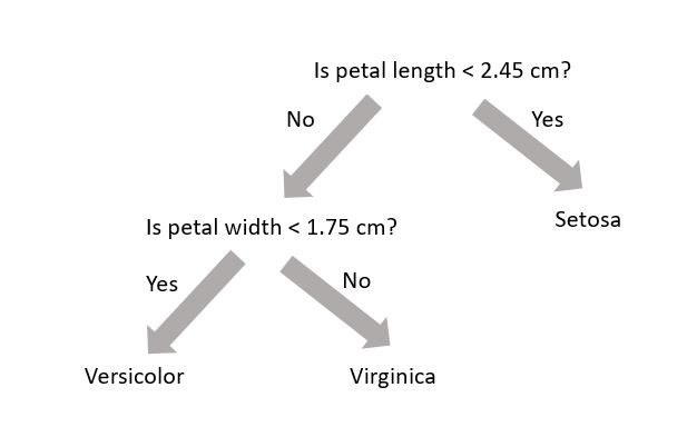
A decision tree is not trained using gradient descent and a loss function; training is completed using the Classification and Regression Tree (CART) algorithm. While each decision tree is a simple algorithm, a random forest uses ensemble learning with many decision trees to make better predictions. A random forest is considered a black-box model while a decision tree is considered a white-box model.

Model Interpretation: White Box vs. Black Box

Decision trees are intuitive, and their decisions are easy to interpret. Such models are considered white-box models. In contrast, random forests or neural networks are generally considered black-box models. They can make great predictions but it is usually hard to explain in simple terms why the predictions were made. For example, if a neural network says that a particular person appears on a picture, it is hard to know what contributed to that prediction. Was it their mouth? Their nose? Their shoes? Or even the couch they were sitting on? Conversely, decision trees provide nice, simple classification rules that can be applied manually if need be.

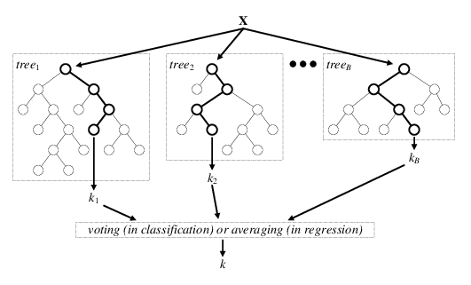
The diagram below is a visual representation of random forests; there are $B$ decision trees and each decision tree $\text{tree}_j$ makes the prediction that a particular data point $x$ belongs to the class $k_j$. Each decision tree has a varying level of confidence in their prediction. Then, using weighted voting, all the predictions $k_1,...k_B$ are considered together to generate a single prediction that the data point $x$ belongs to class $k$.

Random Forest

Wisdom of the Crowd (Ensemble Learning)

Suppose you pose a complex question to thousands of random people, then aggregate their answers. In many cases you will find that this aggregated answer is better than an expert’s answer. This phenomenon is known as wisdom of the crowd. Similarly, if you aggregate the predictions from a group of predictors (such as classifiers or reggressors), you will often get better predictions than with the individual predictor. A group of predictors is called an ensemble. For an interesting example of this phenomenon in estimating the weight of an ox, see this national geographic article.

In the previous page we created a training and test dataset. Lets use these datasets to train a random forest.

from sklearn.ensemble import RandomForestClassifier
from sklearn.metrics import accuracy_score

RF_clf = RandomForestClassifier(
    criterion="gini", max_depth=8, n_estimators=30, random_state=seed_value
)  # initialise your random forest classifier
RF_clf.fit(X_train_scaled, y_train)  # fit to the training data
y_pred_RF = RF_clf.predict(X_test_scaled)  # make predictions on the test data

# See how well the classifier does
print(accuracy_score(y_test, y_pred_RF))

The classifier is created. In this situation we have three hyperparameters specified: criterion, max_depth (max number of consecutive cuts an individual tree can make), and n_estimators (number of decision trees used). These are not altered during training (i.e. they are not included in $\theta$).
The classifier is trained using the training dataset X_train_scaled and corresponding labels y_train. During training, we give the classifier both the features (X_train_scaled) and targets (y_train) and it must learn how to map the data to a prediction. Check out this online article for more info.
The classifier makes predictions on the test dataset X_test_scaled. The machine learning algorithm was not exposed to these data during training.
An accuracy score between the test dataset y_test and machine learning predictions y_pred is made. The accuracy score is defined as the ratio of correctly identified data points to all data points.

Neural Network

A neural network is a black-box model with many hyperparameters. The mathematical structure of neural networks was discussed earlier on in the tutorial. If you are interested and have it available, you can read Chapter 10 of the textbook (and Chapters 11-18 as well, for that matter).

First let’s import the bits we need to build a neural network in PyTorch.

import torch  # import PyTorch
import torch.nn as nn  # import PyTorch neural network
import torch.nn.functional as F  # import PyTorch neural network functional
from torch.autograd import Variable  # create variable from tensor
import torch.utils.data as Data  # create data from tensors

Next we make variables for various PyTorch neural network hyper-parameters:

epochs = 10  # number of training epochs
batch_size = 32  # number of samples per batch
input_size = len(ML_inputs)  # The number of features
num_classes = 2  # The number of output classes. In this case: [signal, background]
hidden_size = 5  # The number of nodes at the hidden layer
learning_rate = 0.001  # The speed of convergence
verbose = True  # flag for printing out stats at each epoch
torch.manual_seed(seed_value)  # set random seed for PyTorch

Now we create tensors, variables, datasets and loaders to build our neural network in PyTorch. We need to keep some events for validation. Validation sets are used to select and tune the final neural network model. Here we’re making use of the PyTorch DataLoader functionality. This is going to be useful later when we want to load data during our training loop.

X_train_tensor = torch.as_tensor(
    X_train_scaled, dtype=torch.float
)  # make tensor from X_train_scaled
y_train_tensor = torch.as_tensor(y_train, dtype=torch.long)  # make tensor from y_train

X_train_var, y_train_var = Variable(X_train_tensor), Variable(
    y_train_tensor
)  # make variables from tensors

X_valid_var, y_valid_var = (
    X_train_var[:100],
    y_train_var[:100],
)  # get first 100 events for validation
X_train_nn_var, y_train_nn_var = (
    X_train_var[100:],
    y_train_var[100:],
)  # get remaining events for training

train_data = Data.TensorDataset(
    X_train_nn_var, y_train_nn_var
)  # create training dataset
valid_data = Data.TensorDataset(X_valid_var, y_valid_var)  # create validation dataset

train_loader = Data.DataLoader(
    dataset=train_data,  # PyTorch Dataset
    batch_size=batch_size,  # how many samples per batch to load
    shuffle=True,
)  # data reshuffled at every epoch

valid_loader = Data.DataLoader(
    dataset=valid_data,  # PyTorch Dataset
    batch_size=batch_size,  # how many samples per batch to load
    shuffle=True,
)  # data reshuffled at every epoch

Here we define the neural network that we’ll be using. This is a simple fully-connected neural network, otherwise known as a multi-layer perceptron (MLP). It has two hidden layers, both with the same number of neurons (hidden_dim). The order of the layers for a forward pass through the network is specified in the forward function. You can see that each fully-connected layer is followed by a ReLU activation function. The function then returns an unnormalised vector of outputs (x; also referred to as logits) and a vector of normalised “probabilities” for x, calculated using the SoftMax function.

class Classifier_MLP(nn.Module):  # define Multi-Layer Perceptron
    def __init__(self, in_dim, hidden_dim, out_dim):  # initialise
        super().__init__()  # lets you avoid referring to the base class explicitly

        self.h1 = nn.Linear(in_dim, hidden_dim)  # hidden layer 1
        self.out = nn.Linear(hidden_dim, out_dim)  # output layer
        self.out_dim = out_dim  # output layer dimension

    def forward(self, x):  # order of the layers

        x = F.relu(self.h1(x))  # relu activation function for hidden layer
        x = self.out(x)  # no activation function for output layer

        return x, F.softmax(x, dim=1)  # SoftMax function

Next we need to specify that we’re using the Classifier_MLP model that we specified above and pass it the parameters it requires (input_size, hidden_dim, out_dim).

We also specify which optimizer we’ll use to train our network. Here I’ve implemented a classic Stochastic Gradient Descent (SGD) optimiser, but there are a wide range of optimizers available in the PyTorch library. For most recent applications the Adam optimizer is used.

NN_clf = Classifier_MLP(
    in_dim=input_size, hidden_dim=hidden_size, out_dim=num_classes
)  # call Classifier_MLP class
optimizer = torch.optim.SGD(
    NN_clf.parameters(), lr=learning_rate
)  # optimize model parameters

The next cell contains the training loop for optimizing the parameters of our neural network. To train the network we loop through the full training data set multiple times. Each loop is called an epoch. However, we don’t read the full dataset all at once in an individual epoch, instead we split it into mini-batches and we use the optimization algorithm to update the network parameters after each batch.

The train_loader that we specified earlier using the PyTorch DataLoader breaks up the full dataset into batches automatically and allows us to load the feature data (x_train) and the label data (y_train) for each batch separately. Moreover, because we specified shuffle=True when we defined the train_loader the full datasets will be shuffled on each epoch, so that we aren’t optimising over an identical sequence of samples in every loop.

PyTorch models (nn.Module) can be set into either training or evaluation mode. For the loop we’ve defined here this setting does not make any difference as we do not use any layers that perform differently during evaluation (e.g. dropout, batch normalisation, etc. ) However, it’s included here for completeness.

_results = []  # define empty list for epoch, train_loss, valid_loss, accuracy
for epoch in range(epochs):  # loop over the dataset multiple times

    # training loop for this epoch
    NN_clf.train()  # set the model into training mode

    train_loss = 0.0  # start training loss counter at 0
    for batch, (x_train_batch, y_train_batch) in enumerate(
        train_loader
    ):  # loop over train_loader

        NN_clf.zero_grad()  # set the gradients to zero before backpropragation because PyTorch accumulates the gradients
        out, prob = NN_clf(
            x_train_batch
        )  # get output and probability on this training batch
        loss = F.cross_entropy(out, y_train_batch)  # calculate loss as cross entropy

        loss.backward()  # compute dloss/dx
        optimizer.step()  # updates the parameters

        train_loss += loss.item() * x_train_batch.size(
            0
        )  # add to counter for training loss

    train_loss /= len(
        train_loader.dataset
    )  # divide train loss by length of train_loader

    if verbose:  # if verbose flag set to True
        print("Epoch: {}, Train Loss: {:4f}".format(epoch, train_loss))

    # validation loop for this epoch:
    NN_clf.eval()  # set the model into evaluation mode
    with torch.no_grad():  # turn off the gradient calculations

        correct = 0
        valid_loss = 0  # start counters for number of correct and validation loss
        for i, (x_valid_batch, y_valid_batch) in enumerate(
            valid_loader
        ):  # loop over validation loader

            out, prob = NN_clf(
                x_valid_batch
            )  # get output and probability on this validation batch
            loss = F.cross_entropy(out, y_valid_batch)  # compute loss as cross entropy

            valid_loss += loss.item() * x_valid_batch.size(
                0
            )  # add to counter for validation loss

            preds = prob.argmax(dim=1, keepdim=True)  # get predictions
            correct += (
                preds.eq(y_valid_batch.view_as(preds)).sum().item()
            )  # count number of correct

        valid_loss /= len(
            valid_loader.dataset
        )  # divide validation loss by length of validation dataset
        accuracy = correct / len(
            valid_loader.dataset
        )  # calculate accuracy as number of correct divided by total

    if verbose:  # if verbose flag set to True
        print(
            "Validation Loss: {:4f}, Validation Accuracy: {:4f}".format(
                valid_loss, accuracy
            )
        )

    # create output row:
    _results.append([epoch, train_loss, valid_loss, accuracy])

results = np.array(_results)  # make array of results
print("Finished Training")
print("Final validation error: ", 100.0 * (1 - accuracy), "%")

The predicted y values for the neural network, y_pred_NN can be obtained like:

X_test_tensor = torch.as_tensor(
    X_test_scaled, dtype=torch.float
)  # make tensor from X_test_scaled
y_test_tensor = torch.as_tensor(y_test, dtype=torch.long)  # make tensor from y_test

X_test_var, y_test_var = Variable(X_test_tensor), Variable(
    y_test_tensor
)  # make variables from tensors

out, prob = NN_clf(X_test_var)  # get output and probabilities from X_test
y_pred_NN = (
    prob.cpu().detach().numpy().argmax(axis=1)
)  # get signal/background predictions

Challenge

Once you have y_pred_NN, see how well your neural network classifier does using accurarcy_score.
Solution
# See how well the classifier does
print(accuracy_score(y_test, y_pred_NN))

The neural network should also have a similar accuracy score to the random forest. Note that while the accuracy is one metric for the strength of a classifier, many other metrics exist as well. We will examine these metrics in the next section.

Accuracy: The Naive Metric

Suppose you have a dataset where 90% of the dataset is background and 10% of the dataset is signal. Now suppose we have a dumb classifier that classifies every data point as background. In this example, the classifier will have 90% accuracy! This demonstrates why accuracy is generally not the preferred performance measure for classifiers, especially when you are dealing with skewed datasets. Skewed datasets show up all the time in high energy physics where one has access to many more background than signal events. In this particular tutorial, we have a dataset with 520000 background events and 165000 signal events.

Your feedback is very welcome! Most helpful for us is if you “Improve this page on GitHub”. If you prefer anonymous feedback, please fill this form.

Key Points

Random forests and neural networks are two viable machine learning models.

Overfitting Check

Overview

Teaching: 5 min
Exercises: 5 min

Questions

How do I check whether my model has overfitted?

Objectives

Determine whether your models are overfitted.

Is there any overfitting?

In this section we will check whether there has been any overfitting during the model training phase. As discussed in the lesson on Mathematical Foundations, overfitting can be an unwanted fly in the ointment, so it should be avoided!

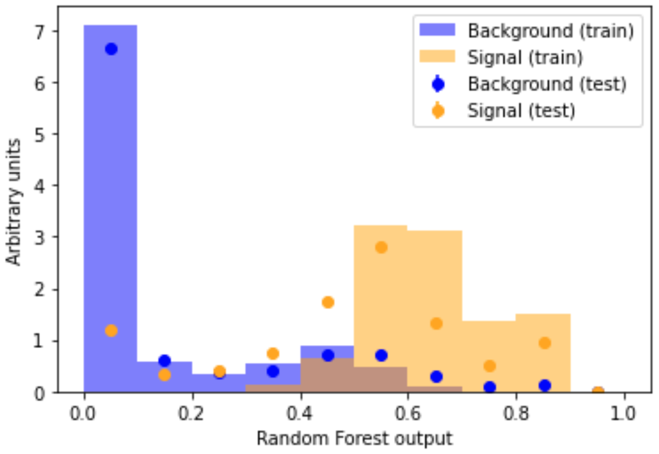
Comparing a machine learning model’s output distribution for the training and testing set is a popular way in High Energy Physics to check for overfitting. The compare_train_test() method will plot the shape of the machine learning model’s decision function for each class, as well as overlaying it with the decision function in the training set.

There are techniques to prevent overfitting.

The code to plot the overfitting check is a bit long, so once again you can see the function definition –>here<–

from my_functions import compare_train_test

compare_train_test(
    RF_clf, X_train_scaled, y_train, X_test_scaled, y_test, "Random Forest output"
)

If overfitting were present, the dots (test set) would be very far from the bars (training set). Look back to the figure in the Overfitting section of the Mathematical Foundations lesson for a brief explanation. Overfitting might look something like this

Overfitted

As discussed in the Mathematical Foundations lesson, there are techniques to prevent overfitting. For instance, you could try reduce the number of parameters in your model, e.g. for a neural network reduce the number of neurons.

Our orange signal dots (test set) nicely overlap with our orange signal histogram bars (training set). The same goes for the blue background. This overlap indicates that no overtaining is present. Happy days!

Challenge

Make the same overfitting check for your neural network and decide whether any overfitting is present.
Solution
compare_train_test(NN_clf, X_train_scaled, y_train, X_test_scaled, y_test, 'Neural Network output')

Now that we’ve checked for overfitting we can go onto comparing our machine learning models!

Your feedback is very welcome! Most helpful for us is if you “Improve this page on GitHub”. If you prefer anonymous feedback, please fill this form.

Key Points

It’s a good idea to check your models for overfitting.

Model Comparison

Overview

Teaching: 10 min
Exercises: 10 min

Questions

How do you use the scikit-learn and PyTorch packages for machine learning?

How do I see whether my machine learning model is doing alright?

Objectives

Check how well our random forest is doing.

Check how well our simple neural network is doing.

Alternative Metrics

As seen in the previous section, accuracy is typically not the preferred metric for classifiers. In this section we will define some new metrics. Let TP, FP, TN, FN be the number of true positives, false positives, true negatives, and false negatives classified using a given model. Note that in this terminology, a background event is considered negative while a signal event is considered positive.

TP: Signal events correctly identified as signal events
FP: Background events incorrectly identified as signal events
TN: Background events correctly identified as background events
FN: Signal events incorrectly identified as background events

Before getting into these metrics, it is important to note that a machine learning binary classifier is capable of providing a probability that a given instance corresponds to a signal or background (i.e. it would output [0.2, 0.8] where the first index corresponds to background and the second index as signal).

Probability or not?

There is some debate as to whether the numbers in the output of a machine learning classifier (such as [0.2, 0.8]) actually represent probabilities. For more information read the following scikit-learn documentation. In general, for a well calibrated classifier, these do in fact represent probabilities in the frequentist interpretation. It can be difficult, however, to assess whether or not a classifier is indeed well calibrated. As such, it may be better to interpret these as confidence levels rather than probabilities.

It is then up to a human user to specify the probability threshold at which something is classified as a signal. For example, you may want the second index to be greater than 0.999 to classify something as a signal. As such, the TP, FP, TN and FN can be altered for a given machine learning classifier based on the threshold requirement for classifying something as a signal event.

Classifiers in Law

In criminal law, Blackstone’s ratio (also known as the Blackstone ratio or Blackstone’s formulation) is the idea that it is better that ten guilty persons escape than that one innocent suffer. This corresponds to the minimum threshold requirement of 91% confidence of a crime being committed for the classification of guilty. It is obviously difficult to get such precise probabilities when dealing with crimes.

Since TP, FP, TN, and FN all depend on the threshold of a classifier, each of these metrics can be considered functions of threshold.

Precision

Precision is defined as

[\text{precision}=\frac{\text{TP}}{\text{TP}+\text{FP}}]

It is the ratio of all things that were correctly classified as positive to all things that were classified as positive. Precision itself is an imperfect metric: a trivial way to have perfect precision is to make one single positive prediction and ensure it is correct (1/1=100%) but this would not be useful. This is equivalent to having a very high threshold. As such, precision is typically combined with another metric: recall.

Recall (True Positive Rate)

Recall is defined as

[\text{recall}=\frac{\text{TP}}{\text{TP}+\text{FN}}]

It is the ratio of all things that were correctly classified as positive to all things that should have been classified as positive. Recall itself is also an imperfect metric: a trivial way to have perfect recall is to classify everything as positive; doing so, however, would result in a poor precision score. This is equivalent to having a very low threshold. As such, precision and recall need to be considered together.

Metrics for our Classifier

By default, the threshold was set to 50% in computing the accuracy score when we made the predictions earlier. For consistency, the threshold is set to 50% here.

from sklearn.metrics import classification_report, roc_auc_score

# Random Forest Report
print(classification_report(y_test, y_pred_RF, target_names=["background", "signal"]))

Challenge

Print the same classification report for your neural network.

Solution

# Neural Network Report
print (classification_report(y_test, y_pred_NN,
                            target_names=["background", "signal"]))

Out of the box, the random forest performs slightly better than the neural network.

Let’s get the decisions of the random forest classifier.

decisions_rf = RF_clf.predict_proba(X_test_scaled)[
    :, 1
]  # get the decisions of the random forest

The decisions of the neural network classifier, decisions_nn, can be obtained like:

decisions_nn = (
    NN_clf(X_test_var)[1][:, 1].cpu().detach().numpy()
)  # get the decisions of the neural network

The ROC Curve

The Receiver Operating Characteristic (ROC) curve is a plot of the recall (or true positive rate) vs. the false positive rate: the ratio of negative instances incorrectly classified as positive. A classifier may classify many instances as positive (i.e. has a low tolerance for classifying something as positive), but in such an example it will probably also incorrectly classify many negative instances as positive as well. The false positive rate is plotted on the x-axis of the ROC curve and the true positive rate on the y-axis; the threshold is varied to give a parametric curve. A random classifier results in a line. Before we look at the ROC curve, let’s examine the following plot

plt.hist(
    decisions_rf[y_test == 0], histtype="step", bins=50, label="Background Events"
)  # plot background
plt.hist(
    decisions_rf[y_test == 1],
    histtype="step",
    bins=50,
    linestyle="dashed",
    label="Signal Events",
)  # plot signal
plt.xlabel("Threshold")  # x-axis label
plt.ylabel("Number of Events")  # y-axis label
plt.semilogy()  # make the y-axis semi-log
plt.legend()  # draw the legend

We can separate this plot into two separate histograms (Higgs vs. non Higgs) because we know beforehand which events correspond to the particular type of event. For real data where the answers aren’t provided, it will be one concatenated histogram. The game here is simple: we pick a threshold (i.e. vertical line on the plot). Once we choose that threshold, everything to the right of that vertical line is classified as a signal event, and everything to the left is classified as a background event. By moving this vertical line left and right (i.e. altering the threshold) we effectively change TP, FP, TN and FN. Hence we also change the true positive rate and the false positive rate by moving this line around.

Suppose we move the threshold from 0 to 1 in steps of 0.01. In doing so, we will get an array of TPRs and FPRs. We can then plot the TPR array vs. the FPR array: this is the ROC curve. To plot the ROC curve, we need to obtain the probabilities that something is classified as a signal (rather than the signal/background prediction itself). This can be done as follows:

from sklearn.metrics import roc_curve

fpr_rf, tpr_rf, thresholds_rf = roc_curve(
    y_test, decisions_rf
)  # get FPRs, TPRs and thresholds for random forest

Challenge

Get the FPRs, TPRs and thresholds for the neural network classifier (fpr_nn, tpr_nn, thresholds_nn).
Solution
fpr_nn, tpr_nn, thresholds_nn = roc_curve(y_test, decisions_nn) # get FPRs, TPRs and thresholds for neural network

Now we plot the ROC curve:

plt.plot(fpr_rf, tpr_rf, label="Random Forest")  # plot random forest ROC
plt.plot(
    fpr_nn, tpr_nn, linestyle="dashed", label="Neural Network"
)  # plot neural network ROC
plt.plot(
    [0, 1], [0, 1], linestyle="dotted", color="grey", label="Luck"
)  # plot diagonal line to indicate luck
plt.xlabel("False Positive Rate")  # x-axis label
plt.ylabel("True Positive Rate")  # y-axis label
plt.grid()  # add a grid to the plot
plt.legend()  # add a legend

(Note: don’t worry if your plot looks slightly different to the video, the classifiers train slightly different each time because they’re random.)

We need to decide on an appropriate threshold.

What Should My Threshold Be?

As discussed above, the threshold depends on the problem at hand. In this specific example of classifying particles as signal or background events, the primary goal is optimizing the discovery region for statistical significance. As discussed here, this metric is the approximate median significance (AMS) defined as

[\text{AMS} = \sqrt{2\left((TPR+FPR+b_r)\ln\left(1+\frac{TPR}{FPR+b_r}\right)-TPR \right)}]

where $TPR$ and $FPR$ are the true and false positive rates and $b_r$ is some number chosen to reduce the variance of the AMS such that the selection region is not too small. For the purpose of this tutorial we will choose $b_r=0.001$. Other values for $b_r$ would also be possible. Once you’ve plotted AMS for the first time, you may want to play around with the value of $b_r$ and see how it affects your selection for the threshold value that maximizes the AMS of the plots. You may see that changing $b_r$ doesn’t change the AMS much.

Challenge

Define a function AMS that calculates AMS using the equation above. Call the true positive rate tpr, false positive rate fpr and $b_r$ b_reg.

Use this function to get the AMS score for your random forest classifier, ams_rf.

Use this function to get the AMS score for your neural network classifier, ams_nn.
Solution to part 1
def AMS(tpr, fpr, b_reg): # define function to calculate AMS
    return np.sqrt(2*((tpr+fpr+b_reg)*np.log(1+tpr/(fpr+b_reg))-tpr)) # equation for AMS
Solution to part 2
ams_rf = AMS(tpr_rf, fpr_rf, 0.001) # get AMS for random forest classifier
Solution to part 3
ams_nn = AMS(tpr_nn, fpr_nn, 0.001) # get AMS for neural network

Then plot:

plt.plot(thresholds_rf, ams_rf, label="Random Forest")  # plot random forest AMS
plt.plot(
    thresholds_nn, ams_nn, linestyle="dashed", label="Neural Network"
)  # plot neural network AMS
plt.xlabel("Threshold")  # x-axis label
plt.ylabel("AMS")  # y-axis label
plt.title("AMS with $b_r=0.001$")  # add plot title
plt.legend()  # add legend

(Note: don’t worry if your plot looks slightly different to the video, the classifiers train slightly different each time because they’re random.)

One should then select the value of the threshold that maximizes the AMS on these plots.

Your feedback is very welcome! Most helpful for us is if you “Improve this page on GitHub”. If you prefer anonymous feedback, please fill this form.

Key Points

Many metrics exist to assess classifier performance.

Making plots is useful to assess classifier performance.

Applying To Experimental Data

Overview

Teaching: 5 min
Exercises: 15 min

Questions

What about real, experimental data?

Are we there yet?

Objectives

Check that our machine learning models behave similarly with real experimental data.

Finish!

What about real, experimental data?

Notice that we’ve trained and tested our machine learning models on simulated data for signal and background. That’s why there are definite labels, y. This has been a case of supervised learning since we knew the labels (y) going into the game. Your machine learning models would then usually be applied to real experimental data once you’re happy with them.

To make sure our machine learning model makes sense when applied to real experimental data, we should check whether simulated data and real experimental data have the same shape in classifier threshold values.

We first need to get the real experimental data.

Challenge to end all challenges

Read data.csv like in the Data Discussion lesson. data.csv is in the same file folder as the files we’ve used so far.

Apply cut_lep_type and cut_lep_charge like in the Data Discussion lesson

Convert the data to a NumPy array, X_data, similar to the Data Preprocessing lesson. You may find the attribute .values useful to convert a pandas DataFrame to a Numpy array.

Don’t forget to transform using the scaler like in the Data Preprocessing lesson. Call the scaled data X_data_scaled.

Predict the labels your random forest classifier would assign to X_data_scaled. Call your predictions y_data_RF.
Solution to part 1
DataFrames['data'] = pd.read_csv('/kaggle/input/4lepton/data.csv') # read data.csv file
Solution to part 2
DataFrames["data"] = DataFrames["data"][
   np.vectorize(cut_lep_type)(
       DataFrames["data"].lep_type_0,
       DataFrames["data"].lep_type_1,
       DataFrames["data"].lep_type_2,
       DataFrames["data"].lep_type_3
   )
]
DataFrames["data"] = DataFrames["data"][
   np.vectorize(cut_lep_charge)(
       DataFrames["data"].lep_charge_0,
       DataFrames["data"].lep_charge_1,
       DataFrames["data"].lep_charge_2,
       DataFrames["data"].lep_charge_3
   )
]
Solution to part 3
X_data = DataFrames['data'][ML_inputs].values # .values converts straight to NumPy array
Solution to part 4
X_data_scaled = scaler.transform(X_data) # X_data now scaled same as training and testing sets
Solution to part 5
y_data_RF = RF_clf.predict(X_data_scaled) # make predictions on the data

Now we can overlay the real experimental data on the simulated data.

labels = ["background", "signal"]  # labels for simulated data
thresholds = (
    []
)  # define list to hold random forest classifier probability predictions for each sample
for s in samples:  # loop over samples
    thresholds.append(
        RF_clf.predict_proba(scaler.transform(DataFrames[s][ML_inputs]))[:, 1]
    )  # predict probabilities for each sample
plt.hist(
    thresholds, bins=np.arange(0, 0.8, 0.1), density=True, stacked=True, label=labels
)  # plot simulated data
data_hist = np.histogram(
    RF_clf.predict_proba(X_data_scaled)[:, 1], bins=np.arange(0, 0.8, 0.1), density=True
)[
    0
]  # histogram the experimental data
scale = sum(RF_clf.predict_proba(X_data_scaled)[:, 1]) / sum(
    data_hist
)  # get scale imposed by density=True
data_err = np.sqrt(data_hist * scale) / scale  # get error on experimental data
plt.errorbar(
    x=np.arange(0.05, 0.75, 0.1), y=data_hist, yerr=data_err, label="Data"
)  # plot the experimental data errorbars
plt.xlabel("Threshold")
plt.legend()

Within errors, the real experimental data errorbars agree with the simulated data histograms. Good news, our random forest classifier model makes sense with real experimental data!

At the end of the day

How many signal events is the random forest classifier predicting?

print(np.count_nonzero(y_data_RF == 1))  # signal

What about background?

print(np.count_nonzero(y_data_RF == 0))  # background

The random forest classifier is predicting how many real data events are signal and how many are background, how cool is that?!

Ready to machine learn to take over the world!

Hopefully you’ve enjoyed this brief discussion on machine learning! Try playing around with the hyperparameters of your random forest and neural network classifiers, such as the number of hidden layers and neurons, and see how they effect the results of your classifiers in Python!

Your feedback is very welcome! Most helpful for us is if you “Improve this page on GitHub”. If you prefer anonymous feedback, please fill this form.

Key Points

It’s a good idea to check whether our machine learning models behave well with real experimental data.

That’s it!

OPTIONAL: TensorFlow

Overview

Teaching: 5 min
Exercises: 15 min

Questions

What other machine learning libraries can I use?

How do classifiers built with different libraries compare?

Objectives

Train a neural network model in TensorFlow.

Compare your TensorFlow neural network with your other classifiers.

TensorFlow

In this section we will examine the fully connected neural network (NN) in TensorFlow, rather than PyTorch.

TensorFlow is an end-to-end open-source platform for machine learning. It is used for building and deploying machine learning models. See the documentation.

TensorFlow does have GPU support, therefore can be used train complicated neural network model that require a lot of GPU power.

TensorFlow is also interoperable with other packages discussed so far, datatypes from NumPy and pandas are often used in TensorFlow.

Here we will import all the required TensorFlow libraries for the rest of the tutorial.

from tensorflow import keras  # tensorflow wrapper
from tensorflow.random import set_seed  # import set_seed function for TensorFlow

set_seed(seed_value)  # set TensorFlow random seed

From the previous pages, we already have our data in NumPy arrays, like X, that can be used in TensorFlow.

Model training

To use a neural network with TensorFlow, we modularize its construction using a function. We will later pass this function into a Keras wrapper.

def build_model(
    n_hidden=1, n_neurons=5, learning_rate=1e-3
):  # function to build a neural network model
    # Build
    model = keras.models.Sequential()  # initialise the model
    for layer in range(n_hidden):  # loop over hidden layers
        model.add(
            keras.layers.Dense(n_neurons, activation="relu")
        )  # add layer to your model
    model.add(keras.layers.Dense(2, activation="softmax"))  # add output layer
    # Compile
    optimizer = keras.optimizers.SGD(
        learning_rate=learning_rate
    )  # define the optimizer
    model.compile(
        loss="sparse_categorical_crossentropy",
        optimizer=optimizer,
        metrics=["accuracy"],
    )  # compile your model
    return model

For now, ignore all the complicated hyperparameters, but note that the loss used is sparse_categorical_crossentropy; the neural network uses gradient descent to optimize its parameters (in this case these parameters are neuron weights).

We need to keep some events for validation. Validation sets are used to select and tune the final neural network model.

X_valid_scaled, X_train_nn_scaled = (
    X_train_scaled[:100],
    X_train_scaled[100:],
)  # first 100 events for validation

Challenge

Assign the first 100 events in y_train for validation (y_valid) and the rest for training your neural network (y_train_nn).
Solution
y_valid, y_train_nn = y_train[:100], y_train[100:] # first 100 events for validation

With these parameters, the network can be trained as follows:

tf_clf = keras.wrappers.scikit_learn.KerasClassifier(
    build_model
)  # call the build_model function defined earlier
tf_clf.fit(
    X_train_nn_scaled, y_train_nn, validation_data=(X_valid_scaled, y_valid)
)  # fit your neural network

Challenge

Get the predicted y values for the TensorFlow neural network, y_pred_tf. Once you have y_pred_tf, see how well your TensorFlow neural network classifier does using accurarcy_score.
Solution
y_pred_tf = tf_clf.predict(X_test_scaled) # make predictions on the test data

# See how well the classifier does
print(accuracy_score(y_test, y_pred_tf))

The TensorFlow neural network should also have a similar accuracy score to the PyTorch neural network.

Overfitting check

Challenge

As shown in the lesson on Overfitting check, make the same overfitting check for your TensorFlow neural network and decide whether any overfitting is present.
Solution
compare_train_test(tf_clf, X_train_nn_scaled, y_train_nn, X_test_scaled, y_test, 'TensorFlow Neural Network output')

Model Comparison

Challenge

Print the same classification report as the Model Comparison lesson for your TensorFlow neural network.
Solution
# TensorFlow Neural Network Report
print (classification_report(y_test, y_pred_tf,
                            target_names=["background", "signal"]))

Challenge

As in the Model Comparison lesson, get the decisions of the TensorFlow neural network classifier, decisions_tf.
Solution
decisions_tf = tf_clf.predict_proba(X_test_scaled)[:,1] # get the decisions of the TensorFlow neural network

ROC curve

Challenge

Get the FPRs, TPRs and thresholds for the TensorFlow neural network classifier (fpr_tf, tpr_tf, thresholds_tf), as was done in the Model Comparison lesson.
Solution
fpr_tf, tpr_tf, thresholds_tf = roc_curve(y_test, decisions_tf) # get FPRs, TPRs and thresholds for TensorFlow neural network

Challenge

Modify your ROC curve plot from the Model Comparison lesson to include another line for the TensorFlow neural network

Solution

plt.plot(fpr_rf, tpr_rf, label='Random Forest') # plot random forest ROC
plt.plot(fpr_nn, tpr_nn, linestyle='dashed', label='PyTorch Neural Network') # plot PyTorch neural network ROC
plt.plot(fpr_tf, tpr_tf, linestyle='dashdot', label='TensorFlow Neural Network') # plot TensorFlow neural network ROC
plt.plot([0, 1], [0, 1], linestyle='dotted', color='grey', label='Luck') # plot diagonal line to indicate luck
plt.xlabel('False Positive Rate') # x-axis label
plt.ylabel('True Positive Rate') # y-axis label
plt.grid() # add a grid to the plot
plt.legend() # add a legend

Threshold

Challenge

Use the function you defined in the Model Comparison lesson to get the AMS score for your TensorFlow neural network classifier, ams_tf.
Solution
ams_tf = AMS(tpr_tf, fpr_tf, 0.001) # get AMS for TensorFlow neural network

Challenge

Modify your threshold plot from the Model Comparison lesson to include another line for the TensorFlow neural network

Solution

plt.plot(thresholds_rf, ams_rf, label='Random Forest') # plot random forest AMS
plt.plot(thresholds_nn, ams_nn, linestyle='dashed', label='PyTorch Neural Network') # plot PyTorch neural network AMS
plt.plot(thresholds_tf, ams_tf, linestyle='dashdot', label='TensorFlow Neural Network') # plot TensorFlow neural network AMS
plt.xlabel('Threshold') # x-axis label
plt.ylabel('AMS') # y-axis label
plt.title('AMS with $b_r=0.001$') # add plot title
plt.legend() # add a legend

All things considered, how does your TensorFlow neural network compare to your PyTorch neural network and scikit-learn random forest?

Your feedback is very welcome! Most helpful for us is if you “Improve this page on GitHub”. If you prefer anonymous feedback, please fill this form.

Key Points

TensorFlow is another good option for machine learning in Python.

OPTIONAL: different dataset

Overview

Teaching: 5 min
Exercises: 35 min

Questions

What other datasets can I use?

How do classifiers perform on different datasets?

Objectives

Train your algorithms on a different dataset.

Compare your algorithms across different datasets.

We’ve already trained some machine learning models on a particular dataset, that for Higgs boson decay to 4 leptons. Now let’s try a different dataset. This will show you the process of using the same algorithms on different datasets. Another thing that will come out of this is that separate optimisation is needed for different datasets.

Data Discussion

New Dataset Used

The new dataset we will use in this tutorial is ATLAS data for a different process. The data were collected with the ATLAS detector at a proton-proton (pp) collision energy of 13 TeV. Monte Carlo (MC) simulation samples are used to model the expected signal and background distributions All samples were processed through the same reconstruction software as used for the data. Each event corresponds to 2 detected leptons and at least 6 detected jets, at least 2 of which are b-tagged jets. Some events correspond to a rare top-quark (signal) process ($t\bar{t}Z$) and others do not (background). Various physical quantities such as jet transverse momentum are reported for each event. The analysis here closely follows this ATLAS published paper studying this rare process.

The signal process is called ‘ttZ’. The background processes are called ‘ttbar’,’Z2HF’,’Z1HF’,’Z0HF’ and ‘Other’.

Challenge

Define a list samples_ttZ containing ‘Other’,’Z1HF’,’Z2HF’,’ttbar’,’ttZ’. (You can add ‘Z0HF’ later). This is similar to samples in the ‘Data Discussion’ lesson.
Solution
samples_ttZ = ['Other','Z1HF','Z2HF','ttbar','ttZ'] # start with only these processes, more can be added later.

Exploring the Dataset

Here we will format the dataset $(x_i, y_i)$ so we can explore! First, we need to open our data set and read it into pandas DataFrames.

Challenge

Define an empty dictionary DataFrames_ttZ to hold your ttZ dataframes. This is similar to DataFrames in the ‘Data Discussion’ lesson.

Loop over samples_ttZ and read the csv files in ‘/kaggle/input/ttz-csv/’ into DataFrames_ttZ. This is similar to reading the csv files in the ‘Data Discussion’ lesson.
Solution
# get data from files
DataFrames_ttZ = {} # define empty dictionary to hold dataframes
for s in samples_ttZ: # loop over samples
    DataFrames_ttZ[s] = pd.read_csv('/kaggle/input/ttz-csv/'+s+".csv") # read .csv file

We’ve already cleaned up this dataset for you and calculated some interesting features, so that you can dive straight into machine learning!

In the ATLAS published paper studying this process, there are 17 variables used in their machine learning algorithms.

Imagine having to separately optimise these 17 variables! Not to mention that applying a cut on one variable could change the distribution of another, which would mean you’d have to re-optimise… Nightmare.

This is where a machine learning model can come to the rescue. A machine learning model can optimise all variables at the same time.

A machine learning model not only optimises cuts, but can find correlations in many dimensions that will give better signal/background classification than individual cuts ever could.

That’s the end of the introduction to why one might want to use a machine learning model. If you’d like to try using one, just keep reading!

Data Preprocessing

Format the data for machine learning

It’s almost time to build a machine learning model!

Challenge

First create a list ML_inputs_ttZ of variables ‘pt4_jet’,’pt6_jet’,’dRll’,’NJetPairsZMass’,’Nmbjj_top’,’MbbPtOrd’,’HT_jet6’,’dRbb’ to use in our machine learning model. (You can add the other variables in later). This is similar to ML_inputs in the ‘Data Preprocessing’ lesson.
Solution
ML_inputs_ttZ = ['pt4_jet','pt6_jet','dRll','NJetPairsZMass','Nmbjj_top','MbbPtOrd','HT_jet6','dRbb'] # list of features for ML model

Definitions of these variables can be found in the ATLAS published paper studying this process.

Challenge

Create an empty list all_MC_ttZ. This is similar to all_MC in the ‘Data Preprocessing’ lesson.

Create an empty list all_y_ttZ. This is similar to all_y in the ‘Data Preprocessing’ lesson.

loop over samples_ttZ. This is similar to looping over samples in the ‘Data Preprocessing’ lesson.

(at each pass through the loop) if currently processing a sample called ‘data’: continue

(at each pass through the loop) append the subset of the DataFrame for this sample containing the columns for ML_inputs_ttZ to to the list all_MC_ttZ. This is similar to the append to all_MC in the ‘Data Preprocessing’ lesson.

(at each pass through the loop) if currently processing a sample called ‘ttZ’: append an array of ones to all_y_ttZ. This is similar to the signal append to all_y in the ‘Data Preprocessing’ lesson.

(at each pass through the loop) else: append an array of zeros to all_y_ttZ. This is similar to the background append to all_y in the ‘Data Preprocessing’ lesson.
Solution to part 1
all_MC_ttZ = [] # define empty list that will contain all features for the MC
Solution to part 2
all_y_ttZ = [] # define empty list that will contain all labels for the MC
Solution to parts 3,4,5,6,7
for s in samples_ttZ: # loop over the different samples
    if s=='data': continue # only MC should pass this
    all_MC_ttZ.append(DataFrames_ttZ[s][ML_inputs_ttZ]) # append the MC dataframe to the list containing all MC features
    if s=='ttZ': all_y_ttZ.append(np.ones(DataFrames_ttZ[s].shape[0])) # signal events are labelled with 1
    else: all_y_ttZ.append(np.zeros(DataFrames_ttZ[s].shape[0])) # background events are labelled 0

Challenge

Run the previous cell and start a new cell.

concatenate the list all_MC_ttZ into an array X_ttZ. This is similar to X in the ‘Data Preprocessing’ lesson.

concatenate the list all_y_ttZ into an array y_ttZ. This is similar to y in the ‘Data Preprocessing’ lesson.
Solution to part 1
X_ttZ = np.concatenate(all_MC_ttZ) # concatenate the list of MC dataframes into a single 2D array of features, called X
Solution to part 2
y_ttZ = np.concatenate(all_y_ttZ) # concatenate the list of labels into a single 1D array of labels, called y

You started from DataFrames and now have a NumPy array consisting of only the DataFrame columns corresponding to ML_inputs_ttZ.

Now we are ready to examine various models $f$ for predicting whether an event corresponds to a signal event or a background event.

Model Training

Random Forest

You’ve just formatted your dataset as arrays. Lets use these datasets to train a random forest. The random forest is constructed and trained against all the contributing backgrounds

Challenge

Define a new RandomForestClassifier called RF_clf_ttZ with max_depth=8,n_estimators=30 as before. This is similar to defining RF_clf in the ‘Model Training’ lesson.

fit your RF_clf_ttZ classifier to X_ttZ and y_ttZ. This is similar to the fit to RF_clf in the ‘Model Training’ lesson.
Solution to part 1
RF_clf_ttZ = RandomForestClassifier(max_depth=8, n_estimators=30) # initialise your random forest classifier
# you may also want to specify criterion, random_seed
Solution to part 2
RF_clf_ttZ.fit(X_ttZ, y_ttZ) # fit to the data

The classifier is created.
The classifier is trained using the dataset X_ttZ and corresponding labels y_ttZ. During training, we give the classifier both the features (X_ttZ) and targets (y_ttZ) and it must learn how to map the data to a prediction. The fit() method returns the trained classifier. When printed out all the hyper-parameters are listed. Check out this online article for more info.

Applying to Experimental Data

We first need to get the real experimental data.

Challenge to end all challenges

Read data.csv like in the Data Discussion lesson. data.csv is in the same file folder as the files we’ve used so far for this new dataset.

Convert the data to a NumPy array, X_data_ttZ, similar to the Data Preprocessing lesson. You may find the attribute .values useful to convert a pandas DataFrame to a Numpy array.

Define an empty list thresholds_ttZ to hold classifier probability predictions for each sample. This is similar to thresholds in the ‘Applying to Experimental Data’ lesson.

Define empty lists weights_ttZ and colors_ttZ to hold weights and colors for each sample. Simulated events are weighted so that the object identification, reconstruction and trigger efficiencies, energy scales and energy resolutions match those determined from data control samples.
Solution to part 1
DataFrames_ttZ['data'] = pd.read_csv('/kaggle/input/ttz-csv/data.csv') # read data.csv file
Solution to part 2
X_data_ttZ = DataFrames_ttZ['data'][ML_inputs_ttZ].values # .values converts straight to NumPy array
Solution to part 3
thresholds_ttZ = [] # define list to hold classifier probability predictions for each sample
Solution to part 4
weights_ttZ = [] # define list to hold weights for each simulated sample
colors_ttZ = [] # define list to hold colors for each sample being plotted

Let’s make a plot where we directly compare real, experimental data with all simulated data.

# dictionary to hold colors for each sample
colors_dict = {
    "Other": "#79b278",
    "Z0HF": "#ce0000",
    "Z1HF": "#ffcccc",
    "Z2HF": "#ff6666",
    "ttbar": "#f8f8f8",
    "ttZ": "#00ccfd",
}

mc_stat_err_squared = np.zeros(
    10
)  # define array to hold the MC statistical uncertainties, 1 zero for each bin
for s in samples_ttZ:  # loop over samples
    X_s = DataFrames_ttZ[s][
        ML_inputs_ttZ
    ]  # get ML_inputs_ttZ columns from DataFrame for this sample
    predicted_prob = RF_clf_ttZ.predict_proba(X_s)  # get probability predictions
    predicted_prob_signal = predicted_prob[
        :, 1
    ]  # 2nd column of predicted_prob corresponds to probability of being signal
    thresholds_ttZ.append(
        predicted_prob_signal
    )  # append predict probabilities for each sample
    weights_ttZ.append(
        DataFrames_ttZ[s]["totalWeight"]
    )  # append weights for each sample
    weights_squared, _ = np.histogram(
        predicted_prob_signal,
        bins=np.arange(0, 1.1, 0.1),
        weights=DataFrames_ttZ[s]["totalWeight"] ** 2,
    )  # square the totalWeights
    mc_stat_err_squared = np.add(
        mc_stat_err_squared, weights_squared
    )  # add weights_squared for s
    colors_ttZ.append(colors_dict[s])  # append colors for each sample
mc_stat_err = np.sqrt(mc_stat_err_squared)  # statistical error on the MC bars

# plot simulated data
mc_heights = plt.hist(
    thresholds_ttZ,
    bins=np.arange(0, 1.1, 0.1),
    weights=weights_ttZ,
    stacked=True,
    label=samples_ttZ,
    color=colors_ttZ,
)

mc_tot = mc_heights[0][-1]  # stacked simulated data y-axis value

# plot the statistical uncertainty
plt.bar(
    np.arange(0.05, 1.05, 0.1),  # x
    2 * mc_stat_err,  # heights
    bottom=mc_tot - mc_stat_err,
    color="none",
    hatch="////",
    width=0.1,
    label="Stat. Unc.",
)

predicted_prob_data = RF_clf_ttZ.predict_proba(
    X_data_ttZ
)  # get probability predictions on data
predicted_prob_data_signal = predicted_prob_data[
    :, 1
]  # 2nd column corresponds to probability of being signal
data_hist_ttZ, _ = np.histogram(
    predicted_prob_data_signal, bins=np.arange(0, 1.1, 0.1)
)  # histogram the experimental data
data_err_ttZ = np.sqrt(data_hist_ttZ)  # get error on experimental data
plt.errorbar(
    x=np.arange(0.05, 1.05, 0.1),
    y=data_hist_ttZ,
    yerr=data_err_ttZ,
    label="Data",
    fmt="ko",
)  # plot the experimental data
plt.xlabel("Threshold")
plt.legend()

Within errors, the real experimental data errorbars agree with the simulated data histograms. Good news, our random forest classifier model makes sense with real experimental data!

This is already looking similar to Figure 10(c) from the ATLAS published paper studying this process. Check you out, recreating science research!

ttZ paper

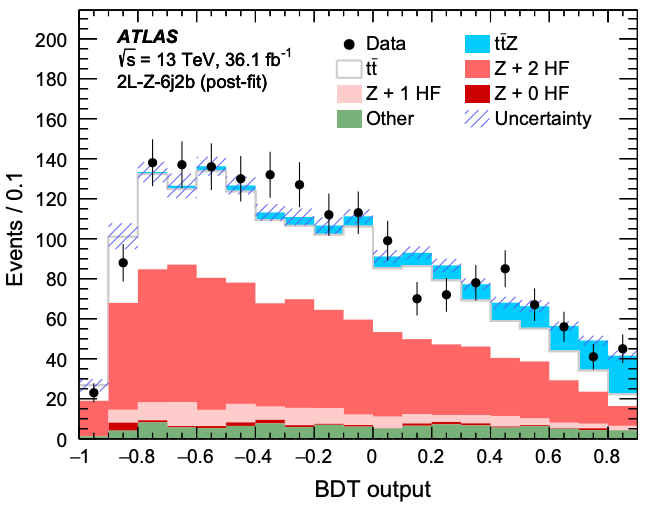
Can you do better? Can you make your graph look more like the published graph? Have we forgotten any steps before applying our machine learning model to data? How would a different machine learning model do?

Here are some suggestions that you could try to go further:

Going further

Add variables into your machine learning models. Start by adding them in the list of ML_inputs_ttZ. See how things look with all variables added.

Add in the other background samples in samples_ttZ by adding the files that aren’t currently being processed. See how things look with all added.

Modify some Random Forest hyper-parameters in your definition of RF_clf_ttZ. You may find the sklearn documentation on RandomForestClassifier helpful.

Give your neural network a go!. Maybe your neural network will perform better on this dataset? You could use PyTorch and/or TensorFlow.

Give a BDT a go!. In the ATLAS published paper studying this process, they used a Boosted Decision Tree (BDT). See if you can use GradientBoostingClassifier rather than RandomForestClassifier.

How important is each variable?. Try create a table similar to the 6j2b column of Table XI of the ATLAS published paper studying this process. feature_importances_ may be useful here.

With each change, keep an eye on the final experimental data graph.

Your feedback is very welcome! Most helpful for us is if you “Improve this page on GitHub”. If you prefer anonymous feedback, please fill this form.

Key Points

The same algorithm can do fairly well across different datasets.

Different optimisation is needed for different datasets.

Introduction to Machine Learning

Introduction

Overview

What is Machine Learning?

What Role Does Machine Learning have in High Energy Physics?

Where to Become Proficient in Machine Learning

Key Points

Mathematical Foundations

Overview

Definitions

Loss Function and Likelihood

Gradient Descent

The Fly in the Ointment: Overfitting

Regression, Classification, Generation

Key Points

Neural Networks

Overview

Neural Network Theory Introduction

TensorFlow Playground

Key Points

Comfort break!

Overview

Key Points

Resources

Overview

Proficiency in Python

Machine Learning Libraries in Python

What about GPUs?

Key Points

Data Discussion

Overview

Code Example

Dataset Used

Exploring the Dataset

Challenge

Solution

Plot some input variables

Challenge

Solution

Key Points

Data Preprocessing

Overview

Format the data for machine learning

Challenge

Solution

Key Points

Comfort break

Overview

Key Points

Model Training

Overview

Models

Random Forest

Model Interpretation: White Box vs. Black Box

Wisdom of the Crowd (Ensemble Learning)

Neural Network

Challenge

Solution

Accuracy: The Naive Metric

Key Points

Overfitting Check

Overview

Is there any overfitting?

Challenge

Solution

Key Points

Model Comparison

Overview

Alternative Metrics

Probability or not?

Classifiers in Law

Precision

Recall (True Positive Rate)

Metrics for our Classifier

Challenge

Solution

The ROC Curve

Challenge

Solution

What Should My Threshold Be?