OPTIONAL: different dataset

Overview

Teaching: 5 min
Exercises: 35 min

Questions

What other datasets can I use?

How do classifiers perform on different datasets?

Objectives

Train your algorithms on a different dataset.

Compare your algorithms across different datasets.

We’ve already trained some machine learning models on a particular dataset, that for Higgs boson decay to 4 leptons. Now let’s try a different dataset. This will show you the process of using the same algorithms on different datasets. Another thing that will come out of this is that separate optimisation is needed for different datasets.

Data Discussion

New Dataset Used

The new dataset we will use in this tutorial is ATLAS data for a different process. The data were collected with the ATLAS detector at a proton-proton (pp) collision energy of 13 TeV. Monte Carlo (MC) simulation samples are used to model the expected signal and background distributions All samples were processed through the same reconstruction software as used for the data. Each event corresponds to 2 detected leptons and at least 6 detected jets, at least 2 of which are b-tagged jets. Some events correspond to a rare top-quark (signal) process (\(t\bar{t}Z\)) and others do not (background). Various physical quantities such as jet transverse momentum are reported for each event. The analysis here closely follows this ATLAS published paper studying this rare process.

The signal process is called ‘ttZ’. The background processes are called ‘ttbar’,’Z2HF’,’Z1HF’,’Z0HF’ and ‘Other’.

Challenge

Define a list samples_ttZ containing ‘Other’,’Z1HF’,’Z2HF’,’ttbar’,’ttZ’. (You can add ‘Z0HF’ later). This is similar to samples in the ‘Data Discussion’ lesson.
Solution
samples_ttZ = ['Other','Z1HF','Z2HF','ttbar','ttZ'] # start with only these processes, more can be added later.

Exploring the Dataset

Here we will format the dataset \((x_i, y_i)\) so we can explore! First, we need to open our data set and read it into pandas DataFrames.

Challenge

Define an empty dictionary DataFrames_ttZ to hold your ttZ dataframes. This is similar to DataFrames in the ‘Data Discussion’ lesson.

Loop over samples_ttZ and read the csv files in ‘/kaggle/input/ttz-csv/’ into DataFrames_ttZ. This is similar to reading the csv files in the ‘Data Discussion’ lesson.
Solution
# get data from files
DataFrames_ttZ = {} # define empty dictionary to hold dataframes
for s in samples_ttZ: # loop over samples
    DataFrames_ttZ[s] = pd.read_csv('/kaggle/input/ttz-csv/'+s+".csv") # read .csv file

We’ve already cleaned up this dataset for you and calculated some interesting features, so that you can dive straight into machine learning!

In the ATLAS published paper studying this process, there are 17 variables used in their machine learning algorithms.

Imagine having to separately optimise these 17 variables! Not to mention that applying a cut on one variable could change the distribution of another, which would mean you’d have to re-optimise… Nightmare.

This is where a machine learning model can come to the rescue. A machine learning model can optimise all variables at the same time.

A machine learning model not only optimises cuts, but can find correlations in many dimensions that will give better signal/background classification than individual cuts ever could.

That’s the end of the introduction to why one might want to use a machine learning model. If you’d like to try using one, just keep reading!

Data Preprocessing

Format the data for machine learning

It’s almost time to build a machine learning model!

Challenge

First create a list ML_inputs_ttZ of variables ‘pt4_jet’,’pt6_jet’,’dRll’,’NJetPairsZMass’,’Nmbjj_top’,’MbbPtOrd’,’HT_jet6’,’dRbb’ to use in our machine learning model. (You can add the other variables in later). This is similar to ML_inputs in the ‘Data Preprocessing’ lesson.
Solution
ML_inputs_ttZ = ['pt4_jet','pt6_jet','dRll','NJetPairsZMass','Nmbjj_top','MbbPtOrd','HT_jet6','dRbb'] # list of features for ML model

Definitions of these variables can be found in the ATLAS published paper studying this process.

The data type is currently a pandas DataFrame: we now need to convert it into a NumPy array so that it can be used in scikit-learn and TensorFlow during the machine learning process. Note that there are many ways that this can be done: in this tutorial we will use the NumPy concatenate functionality to format our data set. For more information, please see the NumPy documentation on concatenate.

Challenge

Create an empty list all_MC_ttZ. This is similar to all_MC in the ‘Data Preprocessing’ lesson.

Create an empty list all_y_ttZ. This is similar to all_y in the ‘Data Preprocessing’ lesson.

loop over samples_ttZ. This is similar to looping over samples in the ‘Data Preprocessing’ lesson.

(at each pass through the loop) if currently processing a sample called ‘data’: continue

(at each pass through the loop) append the subset of the DataFrame for this sample containing the columns for ML_inputs_ttZ to to the list all_MC_ttZ. This is similar to the append to all_MC in the ‘Data Preprocessing’ lesson.

(at each pass through the loop) if currently processing a sample called ‘ttZ’: append an array of ones to all_y_ttZ. This is similar to the signal append to all_y in the ‘Data Preprocessing’ lesson.

(at each pass through the loop) else: append an array of zeros to all_y_ttZ. This is similar to the background append to all_y in the ‘Data Preprocessing’ lesson.
Solution to part 1
all_MC_ttZ = [] # define empty list that will contain all features for the MC
Solution to part 2
all_y_ttZ = [] # define empty list that will contain all labels for the MC
Solution to parts 3,4,5,6,7
for s in samples_ttZ: # loop over the different samples
    if s=='data': continue # only MC should pass this
    all_MC_ttZ.append(DataFrames_ttZ[s][ML_inputs_ttZ]) # append the MC dataframe to the list containing all MC features
    if s=='ttZ': all_y_ttZ.append(np.ones(DataFrames_ttZ[s].shape[0])) # signal events are labelled with 1
    else: all_y_ttZ.append(np.zeros(DataFrames_ttZ[s].shape[0])) # background events are labelled 0

Challenge

Run the previous cell and start a new cell.

concatenate the list all_MC_ttZ into an array X_ttZ. This is similar to X in the ‘Data Preprocessing’ lesson.

concatenate the list all_y_ttZ into an array y_ttZ. This is similar to y in the ‘Data Preprocessing’ lesson.
Solution to part 1
X_ttZ = np.concatenate(all_MC_ttZ) # concatenate the list of MC dataframes into a single 2D array of features, called X
Solution to part 2
y_ttZ = np.concatenate(all_y_ttZ) # concatenate the list of labels into a single 1D array of labels, called y

You started from DataFrames and now have a NumPy array consisting of only the DataFrame columns corresponding to ML_inputs_ttZ.

Now we are ready to examine various models \(f\) for predicting whether an event corresponds to a signal event or a background event.

Model Training

Random Forest

You’ve just formatted your dataset as arrays. Lets use these datasets to train a random forest. The random forest is constructed and trained against all the contributing backgrounds

Challenge

Define a new RandomForestClassifier called RF_clf_ttZ with max_depth=8,n_estimators=30 as before. This is similar to defining RF_clf in the ‘Model Training’ lesson.

fit your RF_clf_ttZ classifier to X_ttZ and y_ttZ. This is similar to the fit to RF_clf in the ‘Model Training’ lesson.
Solution to part 1
RF_clf_ttZ = RandomForestClassifier(max_depth=8, n_estimators=30) # initialise your random forest classifier
# you may also want to specify criterion, random_seed
Solution to part 2
RF_clf_ttZ.fit(X_ttZ, y_ttZ) # fit to the data

The classifier is created.
The classifier is trained using the dataset X_ttZ and corresponding labels y_ttZ. During training, we give the classifier both the features (X_ttZ) and targets (y_ttZ) and it must learn how to map the data to a prediction. The fit() method returns the trained classifier. When printed out all the hyper-parameters are listed. Check out this online article for more info.

Applying to Experimental Data

We first need to get the real experimental data.

Challenge to end all challenges

Read data.csv like in the Data Discussion lesson. data.csv is in the same file folder as the files we’ve used so far for this new dataset.

Convert the data to a NumPy array, X_data_ttZ, similar to the Data Preprocessing lesson. You may find the attribute .values useful to convert a pandas DataFrame to a Numpy array.

Define an empty list thresholds_ttZ to hold classifier probability predictions for each sample. This is similar to thresholds in the ‘Applying to Experimental Data’ lesson.

Define empty lists weights_ttZ and colors_ttZ to hold weights and colors for each sample. Simulated events are weighted so that the object identification, reconstruction and trigger efficiencies, energy scales and energy resolutions match those determined from data control samples.
Solution to part 1
DataFrames_ttZ['data'] = pd.read_csv('/kaggle/input/ttz-csv/data.csv') # read data.csv file
Solution to part 2
X_data_ttZ = DataFrames_ttZ['data'][ML_inputs_ttZ].values # .values converts straight to NumPy array
Solution to part 3
thresholds_ttZ = [] # define list to hold classifier probability predictions for each sample
Solution to part 4
weights_ttZ = [] # define list to hold weights for each simulated sample
colors_ttZ = [] # define list to hold colors for each sample being plotted

Let’s make a plot where we directly compare real, experimental data with all simulated data.

# dictionary to hold colors for each sample
colors_dict = {
    "Other": "#79b278",
    "Z0HF": "#ce0000",
    "Z1HF": "#ffcccc",
    "Z2HF": "#ff6666",
    "ttbar": "#f8f8f8",
    "ttZ": "#00ccfd",
}

mc_stat_err_squared = np.zeros(
    10
)  # define array to hold the MC statistical uncertainties, 1 zero for each bin
for s in samples_ttZ:  # loop over samples
    X_s = DataFrames_ttZ[s][
        ML_inputs_ttZ
    ]  # get ML_inputs_ttZ columns from DataFrame for this sample
    predicted_prob = RF_clf_ttZ.predict_proba(X_s)  # get probability predictions
    predicted_prob_signal = predicted_prob[
        :, 1
    ]  # 2nd column of predicted_prob corresponds to probability of being signal
    thresholds_ttZ.append(
        predicted_prob_signal
    )  # append predict probabilities for each sample
    weights_ttZ.append(
        DataFrames_ttZ[s]["totalWeight"]
    )  # append weights for each sample
    weights_squared, _ = np.histogram(
        predicted_prob_signal,
        bins=np.arange(0, 1.1, 0.1),
        weights=DataFrames_ttZ[s]["totalWeight"] ** 2,
    )  # square the totalWeights
    mc_stat_err_squared = np.add(
        mc_stat_err_squared, weights_squared
    )  # add weights_squared for s
    colors_ttZ.append(colors_dict[s])  # append colors for each sample
mc_stat_err = np.sqrt(mc_stat_err_squared)  # statistical error on the MC bars

# plot simulated data
mc_heights = plt.hist(
    thresholds_ttZ,
    bins=np.arange(0, 1.1, 0.1),
    weights=weights_ttZ,
    stacked=True,
    label=samples_ttZ,
    color=colors_ttZ,
)

mc_tot = mc_heights[0][-1]  # stacked simulated data y-axis value

# plot the statistical uncertainty
plt.bar(
    np.arange(0.05, 1.05, 0.1),  # x
    2 * mc_stat_err,  # heights
    bottom=mc_tot - mc_stat_err,
    color="none",
    hatch="////",
    width=0.1,
    label="Stat. Unc.",
)

predicted_prob_data = RF_clf_ttZ.predict_proba(
    X_data_ttZ
)  # get probability predictions on data
predicted_prob_data_signal = predicted_prob_data[
    :, 1
]  # 2nd column corresponds to probability of being signal
data_hist_ttZ, _ = np.histogram(
    predicted_prob_data_signal, bins=np.arange(0, 1.1, 0.1)
)  # histogram the experimental data
data_err_ttZ = np.sqrt(data_hist_ttZ)  # get error on experimental data
plt.errorbar(
    x=np.arange(0.05, 1.05, 0.1),
    y=data_hist_ttZ,
    yerr=data_err_ttZ,
    label="Data",
    fmt="ko",
)  # plot the experimental data
plt.xlabel("Threshold")
plt.legend()

Within errors, the real experimental data errorbars agree with the simulated data histograms. Good news, our random forest classifier model makes sense with real experimental data!

This is already looking similar to Figure 10(c) from the ATLAS published paper studying this process. Check you out, recreating science research!

ttZ paper

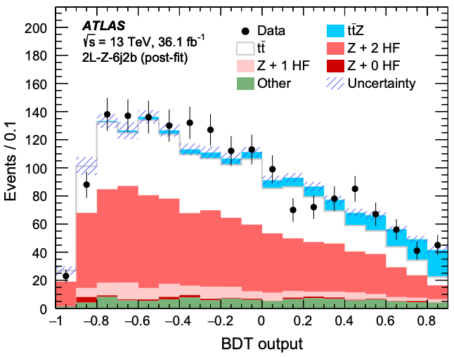
Can you do better? Can you make your graph look more like the published graph? Have we forgotten any steps before applying our machine learning model to data? How would a different machine learning model do?

Here are some suggestions that you could try to go further:

Going further

Add variables into your machine learning models. Start by adding them in the list of ML_inputs_ttZ. See how things look with all variables added.

Add in the other background samples in samples_ttZ by adding the files that aren’t currently being processed. See how things look with all added.

Modify some Random Forest hyper-parameters in your definition of RF_clf_ttZ. You may find the sklearn documentation on RandomForestClassifier helpful.

Give your neural network a go!. Maybe your neural network will perform better on this dataset? You could use PyTorch and/or TensorFlow.

Give a BDT a go!. In the ATLAS published paper studying this process, they used a Boosted Decision Tree (BDT). See if you can use GradientBoostingClassifier rather than RandomForestClassifier.

How important is each variable?. Try create a table similar to the 6j2b column of Table XI of the ATLAS published paper studying this process. feature_importances_ may be useful here.

With each change, keep an eye on the final experimental data graph.

Your feedback is very welcome! Most helpful for us is if you “Improve this page on GitHub”. If you prefer anonymous feedback, please fill this form.

Key Points

The same algorithm can do fairly well across different datasets.

Different optimisation is needed for different datasets.

previous episode

Introduction to Machine Learning

lesson home

OPTIONAL: different dataset

Overview

Data Discussion

New Dataset Used

Challenge

Solution

Exploring the Dataset

Challenge

Solution

Data Preprocessing

Format the data for machine learning

Challenge

Solution

Challenge

Solution to part 1

Solution to part 2

Solution to parts 3,4,5,6,7

Challenge

Solution to part 1

Solution to part 2

Model Training

Random Forest

Challenge

Solution to part 1

Solution to part 2

Applying to Experimental Data

Challenge to end all challenges

Solution to part 1

Solution to part 2

Solution to part 3

Solution to part 4

Going further

Key Points

previous episode

lesson home