Overview

Teaching: 15 min
Exercises: 15 min

Questions

• How does one train machine learning models in Python?

• What machine learning models might be appropriate?

Objectives

• Train a random forest model.

• Train a neural network model.

Models

In this section we will examine 2 different machine learning models \(f\) for classification: the random forest (RF) and the fully connected neural network (NN).

Random Forest

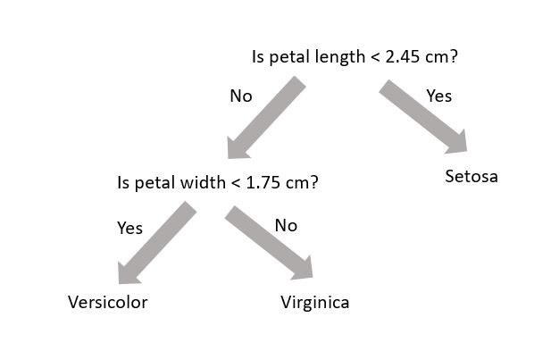
A random forest (see Wikipedia or Chapter 7) uses decision trees (see Wikipedia or Chapter 6) to make predictions. Decision trees are very simple models that make classification predictions by performing selections on regions in the data set. The diagram below shows a decision tree for classifying three different types of iris flower species.

A decision tree is not trained using gradient descent and a loss function; training is completed using the Classification and Regression Tree (CART) algorithm. While each decision tree is a simple algorithm, a random forest uses ensemble learning with many decision trees to make better predictions. A random forest is considered a black-box model while a decision tree is considered a white-box model.

Model Interpretation: White Box vs. Black Box

Decision trees are intuitive, and their decisions are easy to interpret. Such models are considered white-box models. In contrast, random forests or neural networks are generally considered black-box models. They can make great predictions but it is usually hard to explain in simple terms why the predictions were made. For example, if a neural network says that a particular person appears on a picture, it is hard to know what contributed to that prediction. Was it their mouth? Their nose? Their shoes? Or even the couch they were sitting on? Conversely, decision trees provide nice, simple classification rules that can be applied manually if need be.

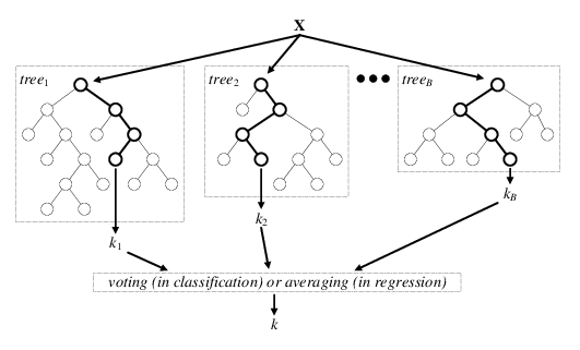
The diagram below is a visual representation of random forests; there are \(B\) decision trees and each decision tree \(\text{tree}_j\) makes the prediction that a particular data point \(x\) belongs to the class \(k_j\). Each decision tree has a varying level of confidence in their prediction. Then, using weighted voting, all the predictions \(k_1,...k_B\) are considered together to generate a single prediction that the data point \(x\) belongs to class \(k\).

Wisdom of the Crowd (Ensemble Learning)

Suppose you pose a complex question to thousands of random people, then aggregate their answers. In many cases you will find that this aggregated answer is better than an expert’s answer. This phenomenon is known as wisdom of the crowd. Similarly, if you aggregate the predictions from a group of predictors (such as classifiers or reggressors), you will often get better predictions than with the individual predictor. A group of predictors is called an ensemble. For an interesting example of this phenomenon in estimating the weight of an ox, see this national geographic article.

In the previous page we created a training and test dataset. Lets use these datasets to train a random forest.

from sklearn.ensemble import RandomForestClassifier
from sklearn.metrics import accuracy_score

RF_clf = RandomForestClassifier(
    criterion="gini", max_depth=8, n_estimators=30, random_state=seed_value
)  # initialise your random forest classifier
RF_clf.fit(X_train_scaled, y_train)  # fit to the training data
y_pred_RF = RF_clf.predict(X_test_scaled)  # make predictions on the test data

# See how well the classifier does
print(accuracy_score(y_test, y_pred_RF))

1. The classifier is created. In this situation we have three hyperparameters specified: criterion, max_depth (max number of consecutive cuts an individual tree can make), and n_estimators (number of decision trees used). These are not altered during training (i.e. they are not included in \(\theta\)).
2. The classifier is trained using the training dataset X_train_scaled and corresponding labels y_train. During training, we give the classifier both the features (X_train_scaled) and targets (y_train) and it must learn how to map the data to a prediction. Check out this online article for more info.
3. The classifier makes predictions on the test dataset X_test_scaled. The machine learning algorithm was not exposed to these data during training.
4. An accuracy score between the test dataset y_test and machine learning predictions y_pred is made. The accuracy score is defined as the ratio of correctly identified data points to all data points.

Neural Network

A neural network is a black-box model with many hyperparameters. The mathematical structure of neural networks was discussed earlier on in the tutorial. If you are interested and have it available, you can read Chapter 10 of the textbook (and Chapters 11-18 as well, for that matter).

First let’s import the bits we need to build a neural network in PyTorch.

import torch  # import PyTorch
import torch.nn as nn  # import PyTorch neural network
import torch.nn.functional as F  # import PyTorch neural network functional
from torch.autograd import Variable  # create variable from tensor
import torch.utils.data as Data  # create data from tensors

Next we make variables for various PyTorch neural network hyper-parameters:

epochs = 10  # number of training epochs
batch_size = 32  # number of samples per batch
input_size = len(ML_inputs)  # The number of features
num_classes = 2  # The number of output classes. In this case: [signal, background]
hidden_size = 5  # The number of nodes at the hidden layer
learning_rate = 0.001  # The speed of convergence
verbose = True  # flag for printing out stats at each epoch
torch.manual_seed(seed_value)  # set random seed for PyTorch

Now we create tensors, variables, datasets and loaders to build our neural network in PyTorch. We need to keep some events for validation. Validation sets are used to select and tune the final neural network model. Here we’re making use of the PyTorch DataLoader functionality. This is going to be useful later when we want to load data during our training loop.

X_train_tensor = torch.as_tensor(
    X_train_scaled, dtype=torch.float
)  # make tensor from X_train_scaled
y_train_tensor = torch.as_tensor(y_train, dtype=torch.long)  # make tensor from y_train

X_train_var, y_train_var = Variable(X_train_tensor), Variable(
    y_train_tensor
)  # make variables from tensors

X_valid_var, y_valid_var = (
    X_train_var[:100],
    y_train_var[:100],
)  # get first 100 events for validation
X_train_nn_var, y_train_nn_var = (
    X_train_var[100:],
    y_train_var[100:],
)  # get remaining events for training

train_data = Data.TensorDataset(
    X_train_nn_var, y_train_nn_var
)  # create training dataset
valid_data = Data.TensorDataset(X_valid_var, y_valid_var)  # create validation dataset

train_loader = Data.DataLoader(
    dataset=train_data,  # PyTorch Dataset
    batch_size=batch_size,  # how many samples per batch to load
    shuffle=True,
)  # data reshuffled at every epoch

valid_loader = Data.DataLoader(
    dataset=valid_data,  # PyTorch Dataset
    batch_size=batch_size,  # how many samples per batch to load
    shuffle=True,
)  # data reshuffled at every epoch

Here we define the neural network that we’ll be using. This is a simple fully-connected neural network, otherwise known as a multi-layer perceptron (MLP). It has two hidden layers, both with the same number of neurons (hidden_dim). The order of the layers for a forward pass through the network is specified in the forward function. You can see that each fully-connected layer is followed by a ReLU activation function. The function then returns an unnormalised vector of outputs (x; also referred to as logits) and a vector of normalised “probabilities” for x, calculated using the SoftMax function.

class Classifier_MLP(nn.Module):  # define Multi-Layer Perceptron
    def __init__(self, in_dim, hidden_dim, out_dim):  # initialise
        super().__init__()  # lets you avoid referring to the base class explicitly

        self.h1 = nn.Linear(in_dim, hidden_dim)  # hidden layer 1
        self.out = nn.Linear(hidden_dim, out_dim)  # output layer
        self.out_dim = out_dim  # output layer dimension

    def forward(self, x):  # order of the layers

        x = F.relu(self.h1(x))  # relu activation function for hidden layer
        x = self.out(x)  # no activation function for output layer

        return x, F.softmax(x, dim=1)  # SoftMax function

Next we need to specify that we’re using the Classifier_MLP model that we specified above and pass it the parameters it requires (input_size, hidden_dim, out_dim).

We also specify which optimizer we’ll use to train our network. Here I’ve implemented a classic Stochastic Gradient Descent (SGD) optimiser, but there are a wide range of optimizers available in the PyTorch library. For most recent applications the Adam optimizer is used.

NN_clf = Classifier_MLP(
    in_dim=input_size, hidden_dim=hidden_size, out_dim=num_classes
)  # call Classifier_MLP class
optimizer = torch.optim.SGD(
    NN_clf.parameters(), lr=learning_rate
)  # optimize model parameters

The next cell contains the training loop for optimizing the parameters of our neural network. To train the network we loop through the full training data set multiple times. Each loop is called an epoch. However, we don’t read the full dataset all at once in an individual epoch, instead we split it into mini-batches and we use the optimization algorithm to update the network parameters after each batch.

The train_loader that we specified earlier using the PyTorch DataLoader breaks up the full dataset into batches automatically and allows us to load the feature data (x_train) and the label data (y_train) for each batch separately. Moreover, because we specified shuffle=True when we defined the train_loader the full datasets will be shuffled on each epoch, so that we aren’t optimising over an identical sequence of samples in every loop.

PyTorch models (nn.Module) can be set into either training or evaluation mode. For the loop we’ve defined here this setting does not make any difference as we do not use any layers that perform differently during evaluation (e.g. dropout, batch normalisation, etc. ) However, it’s included here for completeness.

_results = []  # define empty list for epoch, train_loss, valid_loss, accuracy
for epoch in range(epochs):  # loop over the dataset multiple times

    # training loop for this epoch
    NN_clf.train()  # set the model into training mode

    train_loss = 0.0  # start training loss counter at 0
    for batch, (x_train_batch, y_train_batch) in enumerate(
        train_loader
    ):  # loop over train_loader

        NN_clf.zero_grad()  # set the gradients to zero before backpropragation because PyTorch accumulates the gradients
        out, prob = NN_clf(
            x_train_batch
        )  # get output and probability on this training batch
        loss = F.cross_entropy(out, y_train_batch)  # calculate loss as cross entropy

        loss.backward()  # compute dloss/dx
        optimizer.step()  # updates the parameters

        train_loss += loss.item() * x_train_batch.size(
            0
        )  # add to counter for training loss

    train_loss /= len(
        train_loader.dataset
    )  # divide train loss by length of train_loader

    if verbose:  # if verbose flag set to True
        print("Epoch: {}, Train Loss: {:4f}".format(epoch, train_loss))

    # validation loop for this epoch:
    NN_clf.eval()  # set the model into evaluation mode
    with torch.no_grad():  # turn off the gradient calculations

        correct = 0
        valid_loss = 0  # start counters for number of correct and validation loss
        for i, (x_valid_batch, y_valid_batch) in enumerate(
            valid_loader
        ):  # loop over validation loader

            out, prob = NN_clf(
                x_valid_batch
            )  # get output and probability on this validation batch
            loss = F.cross_entropy(out, y_valid_batch)  # compute loss as cross entropy

            valid_loss += loss.item() * x_valid_batch.size(
                0
            )  # add to counter for validation loss

            preds = prob.argmax(dim=1, keepdim=True)  # get predictions
            correct += (
                preds.eq(y_valid_batch.view_as(preds)).sum().item()
            )  # count number of correct

        valid_loss /= len(
            valid_loader.dataset
        )  # divide validation loss by length of validation dataset
        accuracy = correct / len(
            valid_loader.dataset
        )  # calculate accuracy as number of correct divided by total

    if verbose:  # if verbose flag set to True
        print(
            "Validation Loss: {:4f}, Validation Accuracy: {:4f}".format(
                valid_loss, accuracy
            )
        )

    # create output row:
    _results.append([epoch, train_loss, valid_loss, accuracy])

results = np.array(_results)  # make array of results
print("Finished Training")
print("Final validation error: ", 100.0 * (1 - accuracy), "%")

The predicted y values for the neural network, y_pred_NN can be obtained like:

X_test_tensor = torch.as_tensor(
    X_test_scaled, dtype=torch.float
)  # make tensor from X_test_scaled
y_test_tensor = torch.as_tensor(y_test, dtype=torch.long)  # make tensor from y_test

X_test_var, y_test_var = Variable(X_test_tensor), Variable(
    y_test_tensor
)  # make variables from tensors

out, prob = NN_clf(X_test_var)  # get output and probabilities from X_test
y_pred_NN = (
    prob.cpu().detach().numpy().argmax(axis=1)
)  # get signal/background predictions

Challenge

Once you have y_pred_NN, see how well your neural network classifier does using accurarcy_score.

Solution

# See how well the classifier does
print(accuracy_score(y_test, y_pred_NN))

The neural network should also have a similar accuracy score to the random forest. Note that while the accuracy is one metric for the strength of a classifier, many other metrics exist as well. We will examine these metrics in the next section.

Accuracy: The Naive Metric

Suppose you have a dataset where 90% of the dataset is background and 10% of the dataset is signal. Now suppose we have a dumb classifier that classifies every data point as background. In this example, the classifier will have 90% accuracy! This demonstrates why accuracy is generally not the preferred performance measure for classifiers, especially when you are dealing with skewed datasets. Skewed datasets show up all the time in high energy physics where one has access to many more background than signal events. In this particular tutorial, we have a dataset with 520000 background events and 165000 signal events.

Your feedback is very welcome! Most helpful for us is if you “Improve this page on GitHub”. If you prefer anonymous feedback, please fill this form.

Key Points

• Random forests and neural networks are two viable machine learning models.