Overview

Teaching: 10 min
Exercises: 10 min

Questions

• What is a neural network?

• How can I visualize a neural network?

Objectives

• Examine the structure of a fully connected sequential neural network.

• Look at the TensorFlow neural network Playground to visualize how a neural network works.

Neural Network Theory Introduction

Here we will introduce the mathematics of a neural network. You are likely familiar with the linear transform \(y=Ax+b\) where \(A\) is a matrix (not necessarily square) and \(y\) and \(b\) have the same dimensions and \(x\) may have a different dimension. For example, if \(x\) has dimension \(n\) and \(y\) and \(b\) have dimensions \(m\) then the matrix \(A\) has dimension \(m\) by \(n\).

Now suppose we have some vector \(x_i\) listing some features (height, weight, body fat) and \(y_i\) contains blood pressure and resting heart rate. A simple linear model to predict the label features given the input features is then \(y=Ax+b\) or \(f(x)=Ax+b\). But we can go further. Suppose we also apply a simple but non-linear function \(g\) to the output so that \(f(x) = g(Ax+b)\). This function \(g\) does not change the dimension of \(Ax+b\) as it is an element-wise operation. This function \(g\) is known as an activation function. The activation function defines the output given an input or set of inputs. The purpose of the activation function is to introduce non-linearity into the output (Wikipedia). Non-linearity allows us to describe patterns in data that are more complicated than a straight line. A few activation functions \(g\) are shown below.

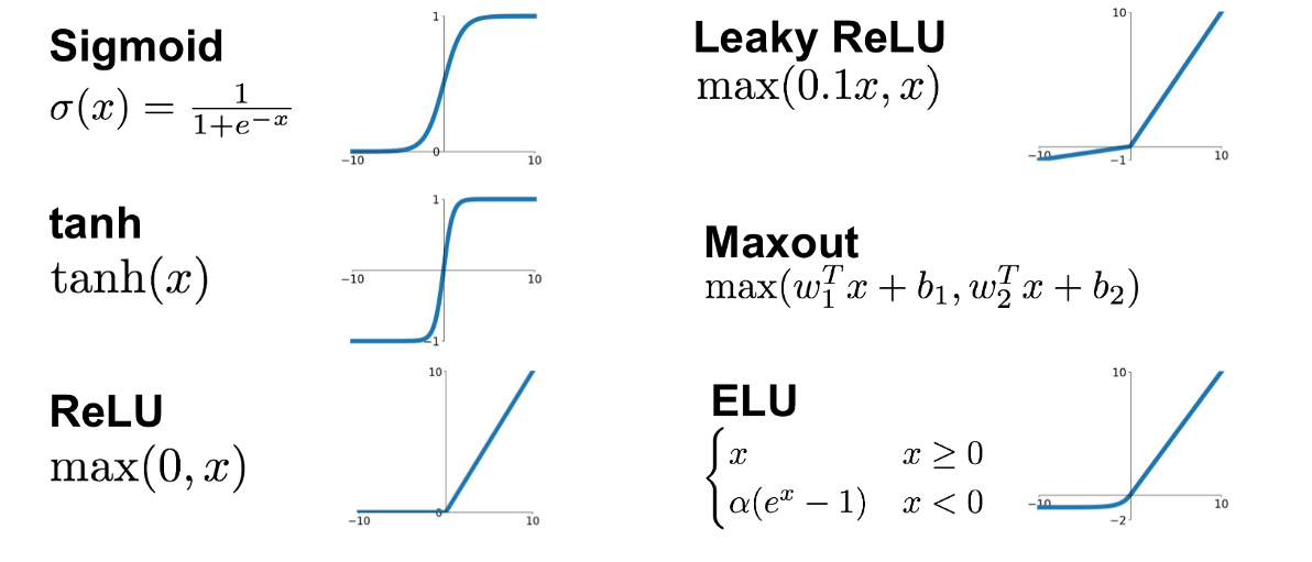
(No general picture is shown for the Maxout function since it depends on the number of w and b used)

Each of these 6 activation functions has different advantages and disadvantages.

Now we can perform a sequence of operations to construct a highly non-linear function. For example; we can construct the following model:

We first perform a linear transformation, then apply activation function \(g_1\), then perform another linear transformation, then apply activation function \(g_2\). The input \(x\) and the output \(f(x)\) are not necessarily the same dimension.

For example, suppose we have an image (which we flatten into a 1d array). This array might be 40000 elements long. If the matrix \(A_1\) has 2000 rows, we can perform one iteration of \(g_1(A_1x+b_1)\) to reduce this to a size of 2000. We can apply this over and over again until eventually only a single value is output. This is the foundation of a fully connected neural network. Note we can also increase the dimensions throughout the process, as seen in the image below. We start with a vector \(x\) of size 3, perform the transformation \(g_1(A_1x+b_1)\) so the vector is size 4, then perform one final transformation so the vector is size 2.

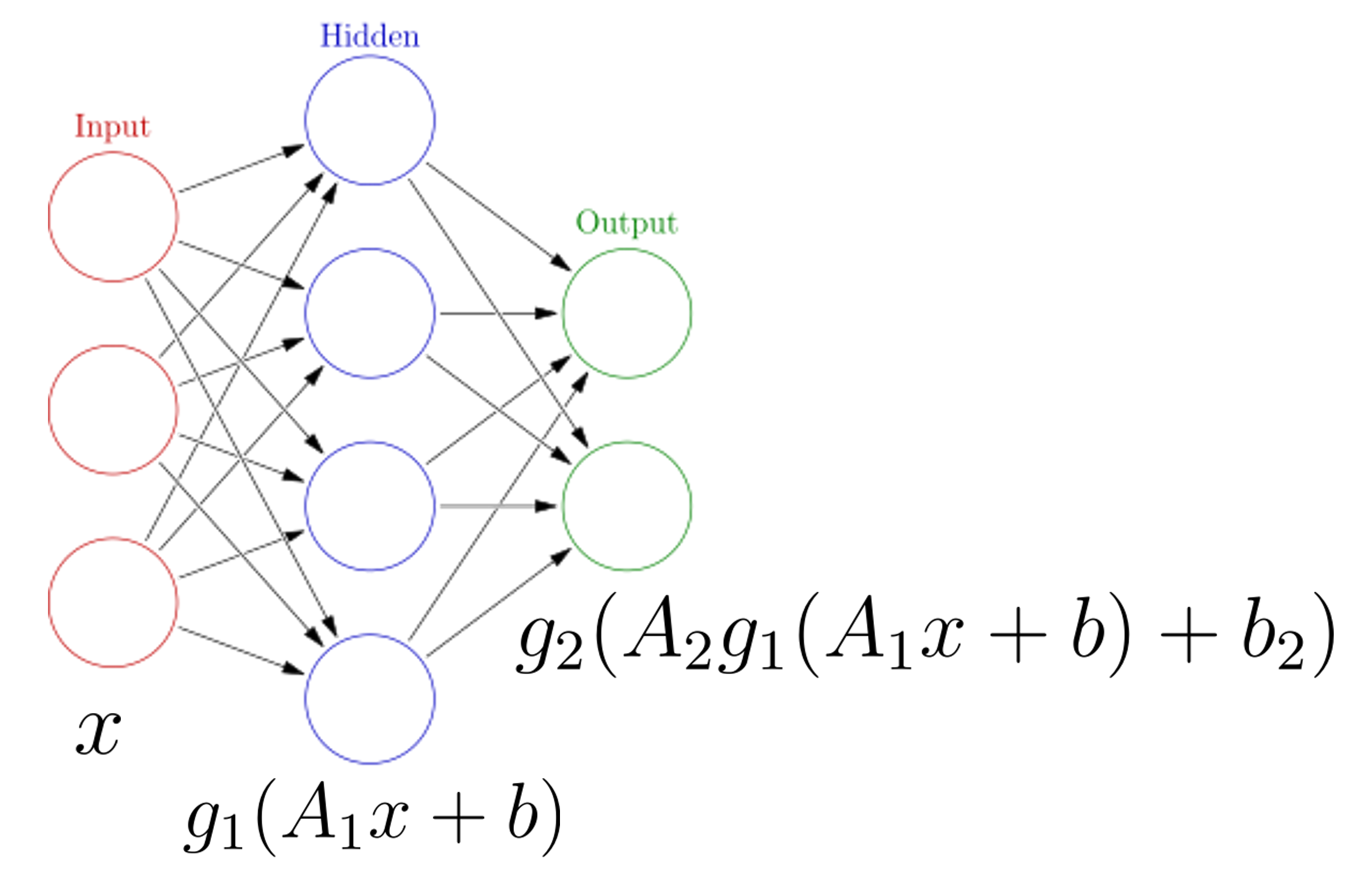
• The vector \(x\) is referred to as the input layer of the network
• Intermediate quantities (such as \(g_1(A_1x+b_1)\)) are referred to as hidden layers. Each element of the vector \(g_1(A_1x+b_1)\) is referred to as a neuron.
• The model output \(f(x)\) is referred to as the output layer. Note that activation functions are generally not used in the output layer.

Neural networks require a careful training procedure. Suppose we are performing a regression task (for example we are given temperature, wind speed, wind direction and pressure, and asked to predict relative humidity). The final output of the neural network will be a single value. During training, we compare the outputs of the neural network \(f(x_i)\) to the true values of the data \(y_i\) using some loss function \(L\). We need to tune the parameters of the model so that \(L\) is as small as possible. What are the parameters of the model in this case? The parameters are the elements of the matrices \(A_1, A_2, ...\) and the vectors \(b_1, b_2, ...\). We also need to adjust them in an appropriate fashion so we are moving closer to the minimum of \(L\). For this we need to compute \(\nabla L\). Using a clever technique known as back-propagation, we can determine exactly how much each parameter (i.e. each entry in matrix \(A_i\)) contributes to \(\nabla L\). Then we slightly adjust each parameter such that \(\vec{L} \to \vec{L}-\alpha \nabla{L}\) where, as before, \(\alpha\) is the learning rate. Through this iterative procedure, we slowly minimize the loss function.

TensorFlow Playground

See here for an interactive example of a neural network structure. Why not play around for about 10 minutes!

Your feedback is very welcome! Most helpful for us is if you “Improve this page on GitHub”. If you prefer anonymous feedback, please fill this form.

Key Points

• Neural networks consist of an input layer, hidden layers and an output layer.

• TensorFlow Playground is a cool place to visualize neural networks!