Autoencoders

Since we explicitly used targets to define the loss function to train neural networks, you may be wondering how they can be unsupervised. They have to be optimized to something; what are they optimized to?

Consider the following neural network:

and suppose that we train it to output the same data that we put in. That is, for each input vector \(\vec{x}_i\), we want the output vector to be as close to \(\vec{x}_i\) as possible. The thing that makes this non-trivial is the fact that an intermediate layer has fewer dimensions than the input/output. All the complexity of data in an 8-dimensional space has to be encoded in a 2-dimensional space.

If the training data just coats a 2-dimensional surface within the 8 dimensions, even as a curvy, potato-shaped submanifold, then the model will learn to flatten it out, so that it can be projected onto the 2-component layer without losing any information. But if the distribution of data extends into 3 or more dimensions, then there will be some information loss, which the model will try to minimize.

This can be thought of as a compression algorithm, but instead of compressing discrete bits into a smaller number of discrete bits, it’s compressing real-valued data into a smaller number of dimensions. (For categorical data in a one-hot encoding, these are essentially the same thing.)

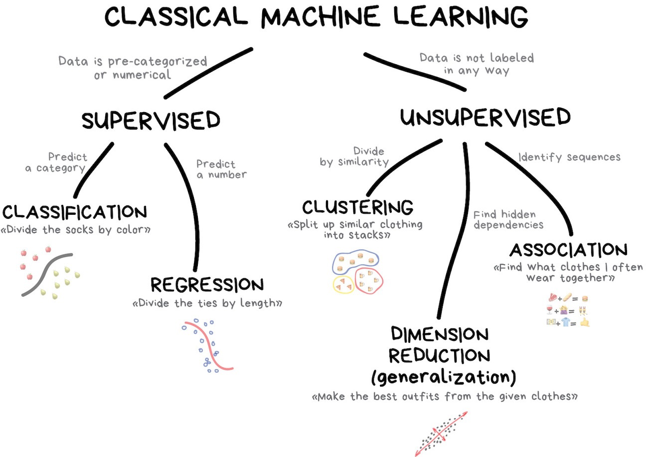
In the diagram from Machine Learning for Everyone, this is “dimension reduction.”

Reducing the number of dimensions is useful for visualization, since humans can visualize at most 3 dimensions, and are much better at visualizing 2 dimensions (as a colored plane) or 1 dimension (as a histogram axis, for instance).

It’s also useful for clustering because in a high-dimensional space, the distances between pairs of points are more nearly equal to each other than in a low-dimensional space (ref). Reducing the number of dimensions is a necessary first step for clustering to be effective, but unlike visualization, the reduced number of dimensions may be higher than 3.

import numpy as np
import pandas as pd
import matplotlib as mpl
import matplotlib.pyplot as plt

import torch
from torch import nn, optim

Training an autoencoder

Let’s use the jet data from the main project.

hls4ml_lhc_jets_hlf = pd.read_parquet("data/hls4ml_lhc_jets_hlf.parquet")
features_unnormalized = torch.tensor(
    hls4ml_lhc_jets_hlf.drop("jet_type", axis=1).values, dtype=torch.float32
)
features = (features_unnormalized - features_unnormalized.mean(axis=0)) / features_unnormalized.std(axis=0)

As a reminder, the jets are characterized by 16 features. Can we compress them into 2 dimensions to make a plot?

features.shape

torch.Size([830000, 16])

Here’s an autoencoder model that takes the 16 dimensions down to 2 in stages:

• 16 inputs → 12 hidden

• 12 hidden → 8 hidden

• 8 hidden → 4 hidden

• 4 hidden → 2 hidden

• make a plot!

• 2 hidden → 4 hidden

• 4 hidden → 8 hidden

• 8 hidden → 12 hidden

• 12 hidden → 16 outputs

class Autoencoder(nn.Module):
    def __init__(self):
        super().__init__()   # let PyTorch do its initialization first

        self.shrinking = nn.Sequential(
            nn.Linear(16, 12),
            nn.Sigmoid(),
            nn.Linear(12, 8),
            nn.Sigmoid(),
            nn.Linear(8, 4),
            nn.Sigmoid(),
            nn.Linear(4, 2),
            nn.Sigmoid(),
        )
        self.growing = nn.Sequential(
            nn.Linear(2, 4),
            nn.Sigmoid(),
            nn.Linear(4, 8),
            nn.Sigmoid(),
            nn.Linear(8, 12),
            nn.Sigmoid(),
            nn.Linear(12, 16),
        )

    def forward(self, features):
        return self.growing(self.shrinking(features))

NUM_EPOCHS = 20
BATCH_SIZE = 500

torch.manual_seed(12345)

model = Autoencoder()

loss_function = nn.MSELoss()

optimizer = optim.Adam(model.parameters(), lr=0.03)

loss_vs_epoch = []
for epoch in range(NUM_EPOCHS):
    total_loss = 0

    for start_batch in range(0, len(features), BATCH_SIZE):
        stop_batch = start_batch + BATCH_SIZE

        optimizer.zero_grad()
    
        predictions = model(features[start_batch:stop_batch])
        loss = loss_function(predictions, features[start_batch:stop_batch])
        total_loss += loss.item()
    
        loss.backward()
        optimizer.step()

    loss_vs_epoch.append(total_loss)
    print(f"{epoch = } {total_loss = }")

epoch = 0 total_loss = 534.906861692667

epoch = 1 total_loss = 351.5135390162468

epoch = 2 total_loss = 339.23160825669765

epoch = 3 total_loss = 363.9568725377321

epoch = 4 total_loss = 338.43476934731007

epoch = 5 total_loss = 305.22689367830753

epoch = 6 total_loss = 282.54971703886986

epoch = 7 total_loss = 249.3524036258459

epoch = 8 total_loss = 217.9524897709489

epoch = 9 total_loss = 193.5910672172904

epoch = 10 total_loss = 179.14277743548155

epoch = 11 total_loss = 173.56490835547447

epoch = 12 total_loss = 167.48046848922968

epoch = 13 total_loss = 164.66360498219728

epoch = 14 total_loss = 162.998711489141

epoch = 15 total_loss = 160.28361170738935

epoch = 16 total_loss = 160.5055928826332

epoch = 17 total_loss = 157.44673538208008

epoch = 18 total_loss = 153.4948441311717

epoch = 19 total_loss = 153.99981369823217

fig, ax = plt.subplots()

ax.plot(range(len(loss_vs_epoch)), loss_vs_epoch)

ax.set_ylim(0, ax.get_ylim()[1])
ax.set_xlabel("epoch")
ax.set_ylabel("loss")

plt.show()

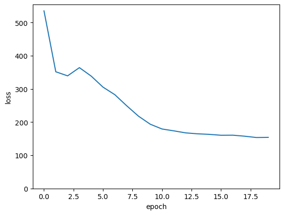
If this were a real project, we’d split the data into training, validation, and test subsamples and try to minimize the loss further. But this is just a demo.

Now let’s look at the distribution of data in the 2-dimensional hidden layer:

embedded = model.shrinking(features).detach().numpy()

fig, ax = plt.subplots(figsize=(6, 5))

xmin, xmax = np.min(embedded[:, 0]), np.max(embedded[:, 0])
ymin, ymax = np.min(embedded[:, 1]), np.max(embedded[:, 1])

def plot_embedded(ax, embedded):    
    p = ax.hist2d(embedded[:, 0], embedded[:, 1],
                  bins=(100, 100), range=((xmin, xmax), (ymin, ymax)),
                  norm=mpl.colors.LogNorm())
    ax.axis([xmin, xmax, ymin, ymax])
    return p

p = plot_embedded(ax, embedded)
fig.colorbar(p[-1], ax=ax, label="number of samples")

plt.show()

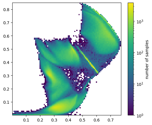
The exact distribution isn’t meaningful (and it would change if we used a different torch.manual_seed). What is relevant is that the optimization process has arranged the data in clumps, presumably for different types of jets, so that it can produce the right distribution in the 16-dimensional feature space.

How well do these clumps correspond to the known jet sources?

hidden_truth = hls4ml_lhc_jets_hlf["jet_type"].values

fig, ax = plt.subplots(5, 1, figsize=(5, 25))

plot_embedded(ax[0], embedded[hidden_truth == "g"])
plot_embedded(ax[1], embedded[hidden_truth == "q"])
plot_embedded(ax[2], embedded[hidden_truth == "t"])
plot_embedded(ax[3], embedded[hidden_truth == "w"])
plot_embedded(ax[4], embedded[hidden_truth == "z"])

ax[0].set_title("gluon jets (\"g\")")
ax[1].set_title("light quark jets (\"q\")")
ax[2].set_title("top quark jets (\"t\")")
ax[3].set_title("W boson jets (\"w\")")
ax[4].set_title("Z boson jets (\"z\")")

plt.show()

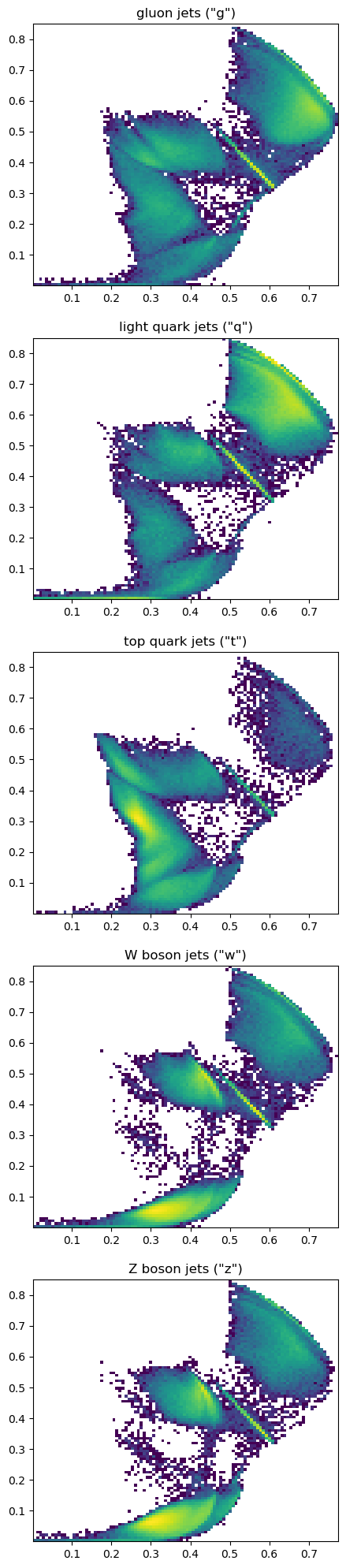
The clumps don’t correspond exactly with jet source, but that’s because jets from the same source can decay in different ways.

Generally, we see the largest differences between gluons/light quarks, top quarks, and \(W\)/\(Z\) bosons, as expected.

To see these as histograms, let’s further compress the 2-dimensional hidden layer to 1 dimension. We can start with the above model as a foundation and zero-out one of its dimensions, then let it optimize around the new restriction.

class Autoencoder1D(nn.Module):
    def __init__(self, shrinking, growing):
        super().__init__()   # let PyTorch do its initialization first

        self.shrinking = shrinking
        self.growing = growing

    def forward(self, features):
        embedded = self.shrinking(features)
        squashed = torch.column_stack([
            embedded[:, [0]],                 # keep the x values, drop the y
            torch.zeros((len(features), 1)),  # make new zeros for y
        ])
        return self.growing(squashed)

NUM_EPOCHS_2 = 20

model1D = Autoencoder1D(model.shrinking, model.growing)

for epoch in range(NUM_EPOCHS_2):
    total_loss = 0

    for start_batch in range(0, len(features), BATCH_SIZE):
        stop_batch = start_batch + BATCH_SIZE

        optimizer.zero_grad()
    
        predictions = model1D(features[start_batch:stop_batch])
        loss = loss_function(predictions, features[start_batch:stop_batch])
        total_loss += loss.item()
    
        loss.backward()
        optimizer.step()

    loss_vs_epoch.append(total_loss)
    print(f"{epoch = } {total_loss = }")

epoch = 0 total_loss = 807.5686780512333

epoch = 1 total_loss = 417.34513951838017

epoch = 2 total_loss = 383.7908398061991

epoch = 3 total_loss = 364.3092810064554

epoch = 4 total_loss = 361.9248836040497

epoch = 5 total_loss = 361.51626697182655

epoch = 6 total_loss = 348.79698772728443

epoch = 7 total_loss = 346.2004083991051

epoch = 8 total_loss = 354.630892470479

epoch = 9 total_loss = 365.76523815095425

epoch = 10 total_loss = 342.19805267453194

epoch = 11 total_loss = 336.74955259263515

epoch = 12 total_loss = 333.2787781059742

epoch = 13 total_loss = 327.2851745188236

epoch = 14 total_loss = 319.50277134776115

epoch = 15 total_loss = 304.4633686840534

epoch = 16 total_loss = 296.406934812665

epoch = 17 total_loss = 296.5493207126856

epoch = 18 total_loss = 295.38260942697525

epoch = 19 total_loss = 300.07434663176537

fig, ax = plt.subplots()

ax.plot(range(len(loss_vs_epoch)), loss_vs_epoch)
ax.axvline(NUM_EPOCHS, color="gray", ls="--")

ax.set_ylim(0, ax.get_ylim()[1])
ax.set_xlabel("epoch")
ax.set_ylabel("loss")

plt.show()

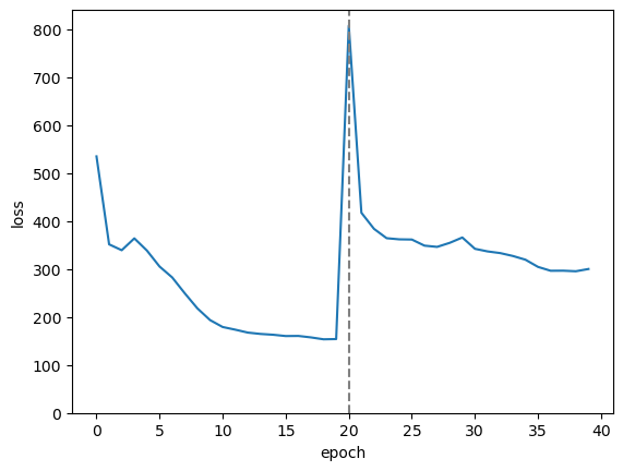
Zeroing-out one of the 2 dimensions made the loss much worse—the model no longer reproduced its input—but a few epochs of iteration allowed this to “heal.”

embedded1D = model1D.shrinking(features).detach().numpy()[:, 0]

fig, ax = plt.subplots()

xmin, xmax = np.min(embedded1D), np.max(embedded1D)

def plot_one(ax, embedded, label):
    ax.hist(embedded, bins=1000, range=(xmin, xmax), histtype="step", label=label)

plot_one(ax, embedded1D[hidden_truth == "g"], "gluon jets (\"g\")")
plot_one(ax, embedded1D[hidden_truth == "q"], "light quark jets (\"q\")")
plot_one(ax, embedded1D[hidden_truth == "t"], "top quark jets (\"t\")")
plot_one(ax, embedded1D[hidden_truth == "w"], "W boson jets (\"w\")")
plot_one(ax, embedded1D[hidden_truth == "z"], "Z boson jets (\"z\")")

ax.set_xlim(xmin, xmax)
ax.set_xlabel("hidden layer value")
ax.set_ylabel("counts")

ax.legend(loc="upper right")

plt.show()

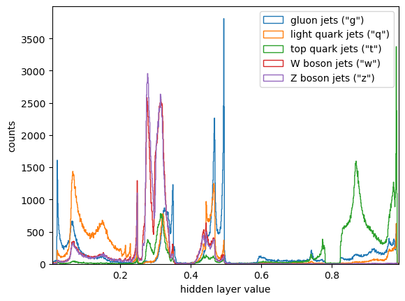
Jets from each of the sources still have a few different ways to decay, but they only partly overlap. Those overlaps are indistinguishable decays (indistinguishable to the current state of the model, at least). But each type also has distinguishable decays.

If our only interest is to identify jet sources and we have the MC truth labels, we’d want to do supervised classification (what you did in your main project). Autoencoders are useful if you don’t have MC truth: for instance, you want to detect any anomalous signal and you don’t know what it would look like before you simulate it.

Self-organizing maps

We used the autoencoder above as a visualization aid, but it’s not the best tool for this job. A self-organizing map is a different neural network topology: instead of a 2-dimensional layer, it outputs \(n\) nodes that are the points of a 2-dimensional grid, and the optimization preserves the topological structure of the data. It produces visualizations that are more stable than the one above.

After reducing the dimensionality of a dataset, we can use the clustering methods from the previous section to categorize the data.

Variational autoencoder

If we plan to cluster the lower-dimensional data with k-means cluster centers \(\vec{c}_j\) or a Gaussian mixture model’s centers \(\vec{\mu}_j\) and covariance matrices \(\hat{\sigma}_j\), why not generate these parameters directly as components of a hidden layer, instead of introducing clustering as a separate step?

This topology is called a variational autoencoder:

In the above, \(\mu_j\), \(\sigma_j\) represent components of cluster centers and covariances. When executing the model, the third layer generates random points with a distribution given by these cluster parameters. Like the basic autoencoder, the variational autoencoder is trained to act as an identity function, returning the vectors \(\vec{x}_i\) close to what it is given as input, but after training, the \(\mu_j\), \(\sigma_j\) parameters can be directly interpreted as peaks and widths of the distribution. This is a neural network with a Gaussian Mixture model built in.