Main Project (2 hours)

Main Project (2 hours)#

In this project, you will download a dataset of jets from a HEP experiment and classify them in 5 categories:

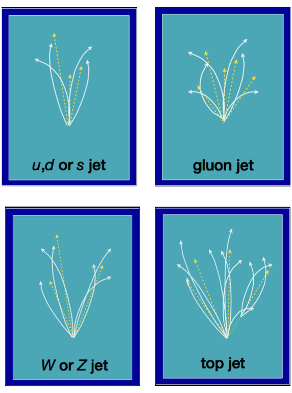
'g': a gluon jet (a gluon from the original proton-proton collision hadronized into a jet)
'q': a light quark hadronized into a jet: up (u), down (d), or strange (s)
't': a top (t) quark decayed into a bottom (b) quark and a W boson, which subsequently decayed and hadronized
'W': a W boson directly from the original proton-proton collision decayed and its constituents hadronized
'Z': the same thing for a Z boson

import numpy as np
import pandas as pd
import matplotlib.pyplot as plt

import torch
from torch import nn, optim
from torch.utils.data import TensorDataset, DataLoader, random_split

Step 1: download and understand the data#

The data comes from an online catalog: hls4ml_lhc_jets_hlf.

The full description is online, with references to the paper in which it was published.

hls4ml_lhc_jets_hlf = pd.read_parquet("data/hls4ml_lhc_jets_hlf.parquet")
features = hls4ml_lhc_jets_hlf.drop("jet_type", axis=1)
targets = hls4ml_lhc_jets_hlf["jet_type"]

View the features (16 numerical properties of jets) as a Pandas DataFrame:

features

	zlogz	c1_b0_mmdt	c1_b1_mmdt	c1_b2_mmdt	c2_b1_mmdt	c2_b2_mmdt	d2_b1_mmdt	d2_b2_mmdt	d2_a1_b1_mmdt	d2_a1_b2_mmdt	m2_b1_mmdt	m2_b2_mmdt	n2_b1_mmdt	n2_b2_mmdt	mass_mmdt	multiplicity
0	-2.935125	0.383155	0.005126	0.000084	0.009070	0.000179	1.769445	2.123898	1.769445	0.308185	0.135687	0.083278	0.412136	0.299058	8.926882	75.0
1	-1.927335	0.270699	0.001585	0.000011	0.003232	0.000029	2.038834	2.563099	2.038834	0.211886	0.063729	0.036310	0.310217	0.226661	3.886512	31.0
2	-3.112147	0.458171	0.097914	0.028588	0.124278	0.038487	1.269254	1.346238	1.269254	0.246488	0.115636	0.079094	0.357559	0.289220	162.144669	61.0
3	-2.666515	0.437068	0.049122	0.007978	0.047477	0.004802	0.966505	0.601864	0.966505	0.160756	0.082196	0.033311	0.238871	0.094516	91.258934	39.0
4	-2.484843	0.428981	0.041786	0.006110	0.023066	0.001123	0.552002	0.183821	0.552002	0.084338	0.048006	0.014450	0.141906	0.036665	79.725777	35.0
...	...	...	...	...	...	...	...	...	...	...	...	...	...	...	...	...
829995	-3.575320	0.473246	0.040693	0.005605	0.053711	0.004402	1.319914	0.785488	1.319914	0.211968	0.106151	0.037546	0.315867	0.123637	72.537308	71.0
829996	-2.408292	0.429539	0.040022	0.005620	0.020352	0.000804	0.508506	0.143106	0.508506	0.077383	0.043065	0.011398	0.131738	0.028787	77.263367	30.0
829997	-3.338864	0.467011	0.075235	0.017644	0.097954	0.022681	1.301970	1.285501	1.301970	0.236583	0.110919	0.068624	0.307230	0.183485	136.165955	72.0
829998	-1.535967	0.335411	0.002537	0.000021	0.002692	0.000017	1.061160	0.797847	1.061160	0.175014	0.086063	0.048476	0.271106	0.161818	4.660848	11.0
829999	-2.987995	0.455648	0.005218	0.000073	0.006994	0.000099	1.340265	1.357867	1.340265	0.305734	0.158129	0.092861	0.397832	0.257965	11.555076	42.0

830000 rows × 16 columns

And some summary statistics for each feature:

features.describe()

	zlogz	c1_b0_mmdt	c1_b1_mmdt	c1_b2_mmdt	c2_b1_mmdt	c2_b2_mmdt	d2_b1_mmdt	d2_b2_mmdt	d2_a1_b1_mmdt	d2_a1_b2_mmdt	m2_b1_mmdt	m2_b2_mmdt	n2_b1_mmdt	n2_b2_mmdt	mass_mmdt	multiplicity
count	830000.000000	830000.000000	830000.000000	8.300000e+05	830000.000000	8.300000e+05	830000.000000	830000.000000	830000.000000	830000.000000	830000.000000	830000.000000	830000.000000	830000.000000	830000.000000	830000.000000
mean	-2.865343	0.433322	0.037766	7.995166e-03	0.045608	7.609470e-03	1.295784	1.083618	1.295784	0.190380	0.090024	0.042460	0.281169	0.143915	75.153610	51.887834
std	0.580389	0.055448	0.029154	9.402567e-03	0.038657	1.217365e-02	0.458041	0.730066	0.458041	0.075417	0.036523	0.026396	0.084556	0.080461	55.612557	21.677036
min	-4.759511	0.091104	0.000073	4.472011e-08	0.000002	1.472518e-10	0.005866	0.000156	0.005866	0.000213	0.000077	0.000002	0.000643	0.000018	0.113449	6.000000
25%	-3.283773	0.419295	0.009977	3.371321e-04	0.015352	4.735599e-04	0.976546	0.485602	0.976546	0.125212	0.059285	0.018935	0.213851	0.071025	19.084184	36.000000
50%	-2.909453	0.452219	0.037919	5.950152e-03	0.036848	2.501090e-03	1.278506	0.983084	1.278506	0.192994	0.089061	0.038755	0.292299	0.139280	80.106373	48.000000
75%	-2.493677	0.468801	0.048510	8.193400e-03	0.062181	7.816279e-03	1.559999	1.505659	1.559999	0.251016	0.118213	0.062612	0.350496	0.210668	93.843903	64.000000
max	-0.438996	0.493779	0.165237	7.122659e-02	0.219034	1.079140e-01	3.968144	6.408456	3.968144	0.366573	0.187837	0.137693	0.449523	0.337616	573.616516	212.000000

You can convert the (830000 row × 16 column) DataFrame into a NumPy array (of shape (830000, 16)) with

features.values

array([[-2.93512535e+00,  3.83155316e-01,  5.12587558e-03, ...,
         2.99057871e-01,  8.92688179e+00,  7.50000000e+01],
       [-1.92733514e+00,  2.70698756e-01,  1.58540264e-03, ...,
         2.26661310e-01,  3.88651156e+00,  3.10000000e+01],
       [-3.11214662e+00,  4.58171129e-01,  9.79138538e-02, ...,
         2.89219588e-01,  1.62144669e+02,  6.10000000e+01],
       ...,
       [-3.33886433e+00,  4.67011213e-01,  7.52350464e-02, ...,
         1.83485478e-01,  1.36165955e+02,  7.20000000e+01],
       [-1.53596663e+00,  3.35411340e-01,  2.53672758e-03, ...,
         1.61818489e-01,  4.66084814e+00,  1.10000000e+01],
       [-2.98799491e+00,  4.55647677e-01,  5.21810818e-03, ...,
         2.57964820e-01,  1.15550756e+01,  4.20000000e+01]],
      shape=(830000, 16))

Similarly, you can view the target (5 jet categories) as a Pandas Series:

targets

0         g
1         w
2         t
3         z
4         w
         ..
829995    z
829996    w
829997    t
829998    q
829999    g
Name: jet_type, Length: 830000, dtype: category
Categories (5, object): ['g', 'q', 't', 'w', 'z']

The categories are represented as 5 Python strings (dtype='object' means Python objects in a NumPy array/Pandas Series).

targets.cat.categories

Index(['g', 'q', 't', 'w', 'z'], dtype='object')

But the large dataset consists of (8-bit) integers corresponding to the position in this list of categories.

targets.cat.codes

0         0
1         3
2         2
3         4
4         3
         ..
829995    4
829996    3
829997    2
829998    1
829999    0
Length: 830000, dtype: int8

targets.cat.codes.values

array([0, 3, 2, ..., 2, 1, 0], shape=(830000,), dtype=int8)

As with any new dataset, take some time to explore it, plotting features for each of the categories to see if and how much they overlap, what their general distributions are, etc. You always want to have some sense of the data’s distribution before applying a machine learning algorithm (or any other mechanical procedure).

Step 2: split the data into training, validation, and test samples#

For this exercise, put

80% of the data into the training sample, which the optimizer will use in its fits
10% of the data into the validation sample, which you will look at while developing the model
10% of the data into the test sample, which you should not look at until you’re done and making the final ROC curve

These data are supposed to be Independent and Identically Distributed (IID), but just in case there are any beginning-of-dataset, end-of-dataset biases, sample them randomly.

Remember that PyTorch has a random_split function that you can use with TensorDataset and DataLoader.

Do not look at any goodness-of-fit criteria on the test sample until you are completely done!

Step 3: build a classifier neural network#

Make it have the following architecture:

input 16 numerical features,
pass through 3 (fully connected) hidden layers with 32 vector components each,
ReLU activation functions in each hidden layer,
return probabilities for the 5 output categories. For each input, all of the output probabilities are non-negative and add up to \(1\).

Use any tools you have to improve the quality of the model, but the model should be implemented in PyTorch.

Think about all of the issues covered in the previous sections of this course.

If you use nn.CrossEntropyLoss (that’s not the only way!), remember that it applies a softmax to predicted values you give it, so your model can’t also apply a softmax, and it can take the target values as a 1-dimensional array of integers (the true category) or as a 2-dimensional array of one-hot vectors (the category probabilities, which are all 0’s and 1’s).

Since all of the examples we have seen so far involved small datasets, we used an excessive number of epochs. For this large dataset, you shouldn’t need more than 10 epochs, and it can be useful to debug your model one epoch at a time. Print out useful information in the loop over epochs, so that you don’t have to wait for the whole thing to finish.

Helpful hint: are the input data close to the \((-1, 1)\) interval? If not, what should you do?

Step 4: monitor the loss function#

Plot the loss function versus epoch for the training sample and the validation sample (and not the test sample!).

Do they diverge? If so, what can you do about that?

Suggestion: compute the validation loss before the training loss, since a training loop over mini-batches changes the model state.

Helpful hint: since you’ll be comparing losses computed from different dataset sizes, you need to scale them by the number of data points.

for epoch in range(NUM_EPOCHS):
    features_tensor, targets_tensor = the_validation_sample
    ...
    validation_loss = loss.item() * len(the_validation_sample) * (0.8 / 0.1)

    training_loss = 0
    for features_tensor, targets_tensor in training_sample_batches:
        ...
        training_loss += loss.item() * len(targets_tensor)   # one training mini-batch

Step 5: compute a 5×5 confusion matrix#

Since you have 5 categories, rather than 2, the confusion matrix is 5×5:

	actually `'g'`	actually `'q'`	actually `'t'`	actually `'w'`	actually `'z'`
predicted `'g'`	#	#	#	#	#
predicted `'q'`	#	#	#	#	#
predicted `'t'`	#	#	#	#	#
predicted `'w'`	#	#	#	#	#
predicted `'z'`	#	#	#	#	#

Each prediction from your model is a vector of 5 numbers. The softmax of these 5 numbers are the 5 probabilities for each category (guaranteed by the definition of softmax to add up to 1). If you use nn.CrossEntropyLoss, your model does not apply the softmax, so you’d need to apply it as an additional step.

For a large set of predictions (a 2-dimensional array with shape (num_predictions, 5)), the torch.argmax with axis=1 finds the index of the maximum probability in each prediction.

Use this to count how many true 'g' your model predicts as 'g', how many true 'g' your model predicts as 'q', etc. for all 25 elements of the confusion matrix.

Then plot this matrix as a colormap using Matplotlib’s ax.imshow.

Use the validation sample only!

Step 6: project it down to a 2×2 confusion matrix#

Suppose that we’re primarily interested in how the model separates lightweight QCD jets ('g' and 'q') from heavy electroweak jets ('t', 'w', 'z'). Since the categories are

targets.cat.categories

Index(['g', 'q', 't', 'w', 'z'], dtype='object')

the index range 0:2 selects lightweight QCD probabilities and the index range 2:5 selects heavy electroweak probabilities. By summing over one of these ranges (slice the second dimension of your set of predicted probabilities, followed by torch.sum with axis=1), you get its total probability \(p\), and the other range gives \(1 - p\).

Compute the 2×2 confusion matrix for the problem of distinguishing lightweight QCD jets (background) from heavy electroweak jets (signal). You might find this easiest to write as a function of a threshold, with the default threshold being 0.5. Anyway, you’ll need that for the next step.

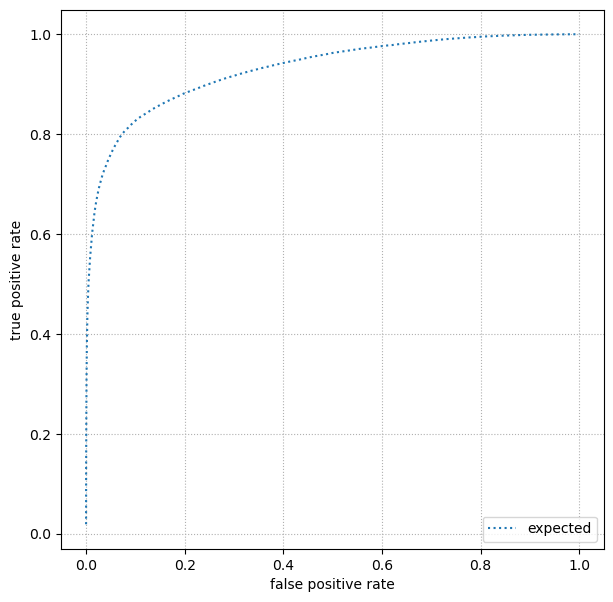
Finally, plot a ROC curve, the true positive rate versus false positive rate curve. How close does your model get to perfection (true positive rate = 1 and false positive rate = 0)? How does its shape differ at one end of the ROC curve from the other? Would it be symmetric if you swapped true positive rate withs false positive rate?

Step 7: plot a ROC curve#

First plot a ROC curve using the validation dataset, and when you’re completely satisfied, finally switch to the test dataset.

Your ROC curve should be close to this one (not exact!):

expected_ROC = np.array([
    [0,               0.01886829927], [0.0001020304051, 0.1289489538],
    [0.0004081216202, 0.209922966  ], [0.0009182736455, 0.3068408332],
    [0.001632486481,  0.376408661  ], [0.002550760127,  0.4303733732],
    [0.003673094582,  0.4678969334 ], [0.004999489848,  0.5027722976],
    [0.006529945924,  0.526339701  ], [0.00826446281,   0.5538282184],
    [0.01020304051,   0.5764214002 ], [0.01234567901,   0.6020473392],
    [0.01469237833,   0.6217746216 ], [0.01724313846,   0.6441249222],
    [0.01999795939,   0.6616243646 ], [0.02295684114,   0.6776505449],
    [0.0261197837,    0.6922878624 ], [0.02948678706,   0.7049561472],
    [0.03305785124,   0.7174712901 ], [0.03683297623,   0.7281837347],
    [0.04081216202,   0.7378146857 ], [0.04499540863,   0.7487390868],
    [0.04938271605,   0.7581570351 ], [0.05397408428,   0.7678773984],
    [0.05876951331,   0.7770101384 ], [0.06376900316,   0.7856509131],
    [0.06897255382,   0.7942924103 ], [0.07438016529,   0.8015956393],
    [0.07999183757,   0.8080126115 ], [0.08580757066,   0.8131647638],
    [0.09182736455,   0.8193828345 ], [0.09805121926,   0.8250768418],
    [0.1044791348,    0.8305736234 ], [0.1111111111,    0.8350616401],
    [0.1179471483,    0.8392843805 ], [0.1249872462,    0.843458635 ],
    [0.132231405,     0.8485805236 ], [0.1396796245,    0.8527170936],
    [0.1473319049,    0.8568358996 ], [0.1551882461,    0.8609808587],
    [0.1632486481,    0.8650308152 ], [0.1715131109,    0.8690270267],
    [0.1799816345,    0.8728376092 ], [0.188654219,     0.8768071621],
    [0.1975308642,    0.8809618493 ], [0.2066115702,    0.8844406165],
    [0.2158963371,    0.8878818684 ], [0.2253851648,    0.8913015608],
    [0.2350780533,    0.895321326  ], [0.2449750026,    0.8988141059],
    [0.2550760127,    0.9023606647 ], [0.2653810836,    0.9060166576],
    [0.2758902153,    0.9095274507 ], [0.2866034078,    0.9131203545],
    [0.2975206612,    0.9160367475 ], [0.3086419753,    0.9194866744],
    [0.3199673503,    0.9227445269 ], [0.331496786,     0.9258525464],
    [0.3432302826,    0.9288425431 ], [0.35516784,      0.9320369642],
    [0.3673094582,    0.934770168  ], [0.3796551372,    0.937793916 ],
    [0.3922048771,    0.9407399938 ], [0.4049586777,    0.9435231388],
    [0.4179165391,    0.946281785  ], [0.4310784614,    0.9488092479],
    [0.4444444444,    0.9518475898 ], [0.4580144883,    0.9547152601],
    [0.471788593,     0.9572437037 ], [0.4857667585,    0.959630249 ],
    [0.4999489848,    0.9625112252 ], [0.5143352719,    0.9647093883],
    [0.5289256198,    0.9668044304 ], [0.5437200286,    0.9689679766],
    [0.5587184981,    0.9712781888 ], [0.5739210285,    0.9728035781],
    [0.5893276196,    0.9748502201 ], [0.6049382716,    0.9769168758],
    [0.6207529844,    0.9783125007 ], [0.636771758,     0.9804721129],
    [0.6529945924,    0.982129956  ], [0.6694214876,    0.9841034064],
    [0.6860524436,    0.9858651034 ], [0.7028874605,    0.9875667363],
    [0.7199265381,    0.9892142364 ], [0.7371696766,    0.9907125562],
    [0.7546168758,    0.9919437219 ], [0.7722681359,    0.9932740291],
    [0.7901234568,    0.9942632436 ], [0.8081828385,    0.9954980595],
    [0.826446281,     0.9962563498 ], [0.8449137843,    0.9970929737],
    [0.8635853484,    0.9977009724 ], [0.8824609734,    0.9984200208],
    [0.9015406591,    0.9988781108 ], [0.9208244057,    0.9991514607],
    [0.940312213,     0.9994587815 ], [0.9600040812,    0.999709012 ],
    [0.9799000102,    0.9998581822 ], [1,               1           ],
])

Overlay your ROC curve on the expected one to see how well you did!

fig, ax = plt.subplots(figsize=(7, 7))

ax.plot(expected_ROC[:, 0], expected_ROC[:, 1], ls=":", color="tab:blue", label="expected")

ax.grid(True, linestyle=":")

ax.set_xlabel("false positive rate")
ax.set_ylabel("true positive rate")

ax.legend(loc="lower right")

plt.show()

_images/7ab376490ab42453823b1b27108f2ab2738cc70ae773e83cbff869e1e79f274f.png