Hyperparameters and validation#
import numpy as np
import pandas as pd
import matplotlib.pyplot as plt

import torch
from torch import nn, optim
Some definitions#
As we’ve seen, the numbers in a model that a minimization algorithm optimizes are called “parameters” (or “weights”):
model = nn.Sequential(
    nn.Linear(5, 5),
    nn.ReLU(),
    nn.Linear(5, 5),
    nn.ReLU(),
    nn.Linear(5, 5),
)
list(model.parameters())
[Parameter containing:
 tensor([[-0.0304, -0.1915, -0.4411,  0.1102,  0.3587],
         [-0.1257, -0.4334,  0.1335, -0.2282, -0.0283],
         [-0.3004, -0.2447,  0.1871,  0.2645, -0.4087],
         [ 0.2120,  0.2539,  0.4086, -0.0222, -0.0601],
         [-0.1936, -0.1136,  0.2533, -0.3331, -0.1497]], requires_grad=True),
 Parameter containing:
 tensor([ 0.1719,  0.1443,  0.0944,  0.0351, -0.2327], requires_grad=True),
 Parameter containing:
 tensor([[-0.4253,  0.2890,  0.1546, -0.2303, -0.3470],
         [-0.3017, -0.2823, -0.3771,  0.1598, -0.1349],
         [ 0.0599, -0.0376,  0.4463, -0.0110,  0.3659],
         [ 0.0391, -0.1536, -0.2454, -0.3294, -0.2809],
         [-0.0165, -0.1544,  0.0017, -0.3511,  0.0572]], requires_grad=True),
 Parameter containing:
 tensor([-0.4032, -0.1268,  0.0141,  0.2505,  0.2020], requires_grad=True),
 Parameter containing:
 tensor([[ 0.2252, -0.3857,  0.3708, -0.3653,  0.0814],
         [-0.1603,  0.2797, -0.2371,  0.3084,  0.0316],
         [-0.1014,  0.1746,  0.1461, -0.2359, -0.0378],
         [ 0.3086,  0.0701,  0.3135, -0.4408,  0.4240],
         [-0.4203,  0.1963, -0.0797, -0.2010, -0.3551]], requires_grad=True),
 Parameter containing:
 tensor([ 0.2046, -0.1847, -0.3444,  0.1753, -0.3374], requires_grad=True)]
I’ve discussed other changeable aspects of models,
architecture (number of hidden layers, how many nodes each, maybe other graph structures),
choice of activation function,
regularization techniques,
choice of input features,
as well as other changeable aspects of the training procedure,
minimization algorithm and its options (such as learning rate and momentum),
distribution of initial parameter values in each layer,
number of epochs and mini-batch size.
It would be confusing to call these choices “parameters,” so we call them “hyperparameters” (“hyper” means “over or above”). The problem of finding the best model is a collaboration between you, the human, choosing hyperparameters and the optimizer choosing parameters. Following the farming analogy from the Overview, the hyperparameters are choices that the farmer gets to make—how much water, how much sun, etc. The parameters are the low-level aspects of how a plant grows, where its leaves branch, how its veins and roots organize themselves to survive. Generally, there are a lot more parameters than hyperparameters.
If there are a lot of hyperparameters to tune, we might want to tune them algorithmically—maybe with a grid search, randomly, or with Bayesian optimization. Technically, I suppose they then become parameters, or we get a three-level hierarchy: parameters, hyperparameters, and hyperhyperparameters! Practitioners might not use consistent terminology (“using ML to tune hyperparameters” is a contradiction in terms), but just don’t get confused about who is optimizing which: algorithm 1, algorithm 2, or human. Even if some hyperparameters are being tuned by an algorithm, some of them must be chosen by hand. For instance, you choose a type of ML algorithm, maybe a neural network, maybe something else, and non-numerical choices about the network topology are generally hand-chosen. If a grid search, random search, or Bayesian optimization is choosing the rest, you do have to set the grid spacing for the grid search, the number of trials and measure of the random search, or various options in the Bayesian search. Or, a software package that you use chooses for you.
Partitioning data into training, validation, and test samples#
In the section on Regularization, we split a dataset into two samples and computed the loss function on each.
Training: loss computed from the training dataset is used to change the parameters of the model. Thus, the loss computed in training can get arbitrarily small as the model is adjusted to fit the training data points exactly (if it has enough parameters to be so flexible).
Test: loss computed from the test dataset acts as an independent measure of the model quality. A model generalizes well if it is a good fit (has minimal loss) on both the training data and data drawn from the same distribution: the test dataset.
Suppose that I set up an ML model with some hand-chosen hyperparameters, optimize it for the training dataset, and then I don’t like how it performs on the test dataset, so I adjust the hyperparameters and run again. And again. After many hyperparameter adjustments, I find a set that optimizes both the training and the test datasets. Is the test dataset an independent measure of the model quality?
It’s not a fair test because my hyperparameter optimization is the same kind of thing as the automated parameter optimization. When I adjust hyperparameters, look at how the loss changes, and use that information to either revert the hyperparameters or make another change, I am acting as a minimization algorithm—just a slow, low-dimensional one.
Since we do need to optimize (some of) the hyperparameters, we need a third data subsample:
Validation: loss computed from the validation dataset is used to change the hyperparameters of the model.
So we need to do a 3-way split of the original dataset. A common practice is to use 80% of the data for training, 10% of the data for validation, and hold 10% of the data for the final test—do not look at its loss value until you’re sure you won’t be changing hyperparameters anymore. This is similar to the practice, in particle physics, of performing a blinded analysis: you can’t look at the analysis result until you are no longer changing the analysis procedure (and then you’re stuck with it).
The fractions, 80%, 10%, 10%, are conventional. They’re not hyperparameters—you can’t change the proportions during model-tuning. Since the validation and test datasets are smallest, their sizes set the resolution of the model evaluation, so you might need to increase them (to, say, 60%, 20%, 20%) if you know that 10% of your data won’t be enough to quantify precision. But if you’re statistics-limited, neural networks might not be the best ML model (consider Boosted Decision Trees (BDTs) instead).
PyTorch’s random_split function can split a dataset into 3 parts as easily as 2.
boston_prices_df = pd.read_csv(
    "data/boston-house-prices.csv", sep="\s+", header=None,
    names=["CRIM", "ZN", "INDUS", "CHAS", "NOX", "RM", "AGE", "DIS", "RAD", "TAX", "PTRATIO", "B", "LSTAT", "MEDV"],
)
boston_prices_df = (boston_prices_df - boston_prices_df.mean()) / boston_prices_df.std()

features = boston_prices_df.drop(columns=["MEDV"])
targets = boston_prices_df["MEDV"]
from torch.utils.data import TensorDataset, DataLoader, random_split
features_tensor = torch.tensor(features.values, dtype=torch.float32)
targets_tensor = torch.tensor(targets.values[:, np.newaxis], dtype=torch.float32)

dataset = TensorDataset(features_tensor, targets_tensor)

train_size = int(np.floor(0.8 * len(dataset)))
valid_size = int(np.floor(0.1 * len(dataset)))
test_size = len(dataset) - train_size - valid_size
train_dataset, valid_dataset, test_dataset = random_split(dataset, [train_size, valid_size, test_size])

len(train_dataset), len(valid_dataset), len(test_dataset)
(404, 50, 52)
Oddly, Scikit-Learn’s equivalent, train_test_split, can only return 2 parts. If you use it, you have to use it like this:
from sklearn.model_selection import train_test_split
train_features, tmp_features, train_targets, tmp_targets = train_test_split(features.values, targets.values, train_size=0.8)
valid_features, test_features, valid_targets, test_targets = train_test_split(tmp_features, tmp_targets, train_size=0.5)

del tmp_features, tmp_targets

len(train_features), len(valid_features), len(test_features)
(404, 51, 51)
although Scikit-Learn does return NumPy arrays or Pandas DataFrames, which are more useful than PyTorch Datasets if you can fit everything into memory.
Cross-validation#
For completeness, I should mention an alternative to allocating a validation dataset: you can cross-validate on a larger subsample of the data. In this method, you still need to isolate a test sample for final evaluation, but you can optimize the parameters and hyperparameters using the same data. The following diagram from Scikit-Learn’s documentation illustrates it well:
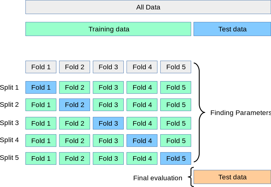
After isolating a test sample, you
subdivide the remaining sample into \(k\) subsamples,
for each \(i \in [0, k)\), combine all data except for subsample \(i\) into a training dataset \(T_i\) and use subsample \(i\) as a validation dataset \(V_i\),
train an independent model on each \(T_i\) and compute the validation loss \(L_i\) with the corresponding trained model and validation dataset \(V_i\),
the total validation loss is \(L = \sum_i L_i\).
This is more computationally expensive, but it makes better use of smaller datasets.
Scikit-Learn provides a KFold object to help keep track of indexes when cross-validating. For \(k = 5\),
from sklearn.model_selection import KFold
kf = KFold(n_splits=5, shuffle=True)
By calling KFold.split on a dataset with a length (that is, an object you can call len on to get its length), you can iterate over folds (\(i \in [0, k)\)) and get random subsamples \(T_i\) and \(V_i\) as arrays of integer indexes.
for train_indexes, valid_indexes in kf.split(dataset):
    print(len(train_indexes), len(valid_indexes))
404 102
405 101
405 101
405 101
405 101
train_indexes[:20]
array([ 0,  1,  3,  4,  5,  6,  7,  8,  9, 11, 13, 14, 15, 16, 17, 18, 19,
       20, 21, 22])
valid_indexes[:20]
array([  2,  10,  12,  29,  30,  31,  36,  46,  59,  60,  61,  63,  64,
        67,  81,  83,  85,  86,  93, 100])
These integer indexes can slice arrays, Pandas DataFrames (via pd.DataFrame.iloc), and PyTorch Tensors.
train_features_i, train_targets_i = dataset[train_indexes]
valid_features_i, valid_targets_i = dataset[valid_indexes]
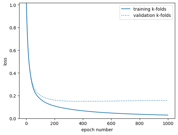
Here’s a full example that computes training loss and validation loss, using cross-validation from the Boston House Prices dataset.
NUMBER_OF_FOLDS = 5
NUMBER_OF_EPOCHS = 1000

kf = KFold(n_splits=NUMBER_OF_FOLDS, shuffle=True)

# use a class so that we can generate new, independent models for every k-fold
class Model(nn.Module):
    def __init__(self):
        super().__init__()   # let PyTorch do its initialization first
        self.model = nn.Sequential(
                nn.Linear(13, 100),
                nn.ReLU(),
                nn.Linear(100, 1),
        )

    def forward(self, x):
        return self.model(x)

# initialize loss-versus-epoch lists as zeros to update with each k-fold
train_loss_vs_epoch = [0] * NUMBER_OF_EPOCHS
valid_loss_vs_epoch = [0] * NUMBER_OF_EPOCHS

# for each k-fold
for train_indexes, valid_indexes in kf.split(dataset):
    train_features_i, train_targets_i = dataset[train_indexes]
    valid_features_i, valid_targets_i = dataset[valid_indexes]

    # generate a new, independent model, loss_function, and optimizer
    model = Model()
    loss_function = nn.MSELoss()
    optimizer = optim.Adam(model.parameters())

    # do a complete training loop
    for epoch in range(NUMBER_OF_EPOCHS):
        optimizer.zero_grad()

        train_loss = loss_function(model(train_features_i), train_targets_i)
        valid_loss = loss_function(model(valid_features_i), valid_targets_i)

        train_loss.backward()
        optimizer.step()

        # average loss over k-folds (could ignore NUMBER_OF_FOLDS to sum, instead)
        train_loss_vs_epoch[epoch] += train_loss.item() / NUMBER_OF_FOLDS
        valid_loss_vs_epoch[epoch] += valid_loss.item() / NUMBER_OF_FOLDS
fig, ax = plt.subplots()

ax.plot(range(1, len(train_loss_vs_epoch) + 1), train_loss_vs_epoch, label="training k-folds")
ax.plot(range(1, len(valid_loss_vs_epoch) + 1), valid_loss_vs_epoch, color="tab:blue", ls=":", label="validation k-folds")

ax.set_ylim(0, min(max(train_loss_vs_epoch), max(valid_loss_vs_epoch)))
ax.set_xlabel("epoch number")
ax.set_ylabel("loss")

ax.legend(loc="upper right")

plt.show()
But since you’ll usually have large datasets (usually Monte Carlo, in HEP), you can usually just split the data 3 ways between training, validation, and test datasets, without mixing training and validation using cross-validation.