Beyond supervised learning: clustering

This course is about deep learning for particle physicists, but so far, its scope has been rather limited:

1. Our neural network examples haven’t been particularly deep, and some of them were linear fits (depth = 0).

2. We’ve dealt with only two types of problems: supervised regression and supervised classification.

3. All of the neural networks we’ve seen have the simplest kind of topology: fully connected, non-recurrent.

The reason for (1) is that making networks deeper is just a matter of adding layers. Deep neural networks used to be hard to train, but many of the technical considerations have been built into the tools we use: backpropagation, initial parameterization, ReLU, Adam, etc. Long computation times and hyperparameter tuning still present challenges, but you can only experience these issues in full-scale problems. This course focuses on understanding the pieces, because that’s what you’ll use to find your way out of such problems.

The reason for (2) is that many (not all) HEP problems are supervised. We usually know what functions we want to approximate because we have detailed Monte Carlo (MC) simulations of the fundamental physics and our detectors, so we can use “MC truth” as targets in training. This is very different from wanting ChatGPT to “respond like a human.” Sometimes, however, particle physicists want algorithms to find unusual events or group points into clusters. These are unsupervised algorithms.

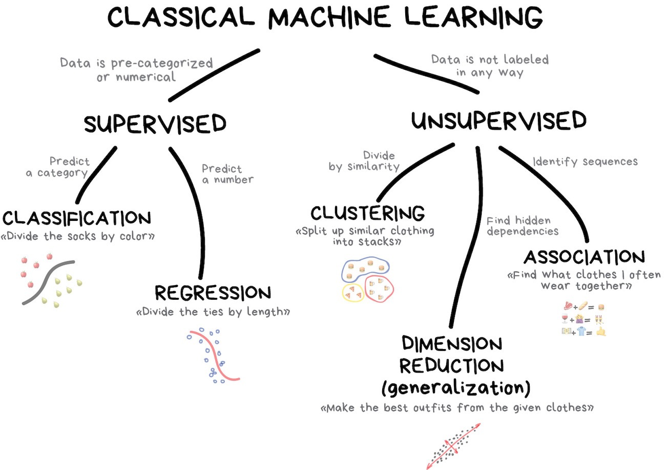
(Diagram from Machine Learning for Everyone.)

For (3), there is no excuse. The fact that neural networks can be arbitrary graphs leaves wide open the question of which topology to use. That’s where much of the research is. In the remainder of this course, we’ll look at a few topologies, but I’ll mostly leave you to explore the neural network zoo on your own.

import numpy as np
import pandas as pd
import matplotlib.pyplot as plt

K-means clustering

Clustering is relatively common in HEP. In a clustering problem, we have a set of features \(\vec{x}_i\) (for \(i \in [0, N)\) and we want to find \(n\) groups or “clusters” of the \(N\) points such that \(\vec{x}_i\) in the same cluster are close to each other and \(\vec{x}_i\) in different clusters are far from each other.

If we know how many clusters we want to make, then the most common choice is k-means clustering. The k-means algorithm starts with \(k\) initial cluster centers, \(\vec{c}_j\) (for \(j \in [0, k)\)) and labels all points in the space of \(\vec{x}\) by the closest cluster: if \(\vec{x}_i\) is closer to \(\vec{c}_j\) than all other \(\vec{c}_{j'}\) (\(j' \ne j\)), then \(\vec{x}_i \in C_j\) where \(C_j\) is the cluster associated with center \(\vec{c}_j\).

The algorithm then moves each cluster center \(\vec{c}_j\) to the mean \(\vec{x}\) for all \(\vec{x} \in C_j\). After enough iterations, the cluster centers gravitate to the densest accumulations of points. Note that this is not a neural network. (We’re getting to that.)

from sklearn.cluster import KMeans

In our penguin classification problem,

penguins_df = pd.read_csv("data/penguins.csv").dropna()
features = penguins_df[["bill_length_mm", "bill_depth_mm"]].values
hidden_truth = penguins_df["species"].values

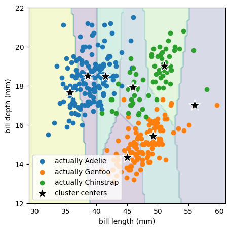
we know there are 3 species of penguins, so let’s try to find 3 clusters.

best_fit = KMeans(3).fit(features)

best_fit.cluster_centers_

array([[38.42426471, 18.27794118],
       [50.90352941, 17.33647059],
       [45.50982143, 15.68303571]])

fig, ax = plt.subplots(figsize=(5, 5))

def plot_clusters(best_fit, xlow=29, xhigh=61, ylow=12, yhigh=22):
    background_x, background_y = np.meshgrid(np.linspace(xlow, xhigh, 100), np.linspace(ylow, yhigh, 100))
    background_2d = np.column_stack([background_x.ravel(), background_y.ravel()])
    ax.contourf(background_x, background_y, best_fit.predict(background_2d).reshape(background_x.shape), alpha=0.2)

    ax.set_xlim(xlow, xhigh)
    ax.set_ylim(ylow, yhigh)

def plot_points(features, hidden_truth):
    ax.scatter(*features[hidden_truth == "Adelie"].T, label="actually Adelie")
    ax.scatter(*features[hidden_truth == "Gentoo"].T, label="actually Gentoo")
    ax.scatter(*features[hidden_truth == "Chinstrap"].T, label="actually Chinstrap")

    ax.set_xlabel("bill length (mm)")
    ax.set_ylabel("bill depth (mm)")

plot_clusters(best_fit)
plot_points(features, hidden_truth)

ax.scatter(*best_fit.cluster_centers_.T, color="white", marker="*", s=300)
ax.scatter(*best_fit.cluster_centers_.T, color="black", marker="*", s=100, label="cluster centers")

ax.legend(loc="lower left")

plt.show()

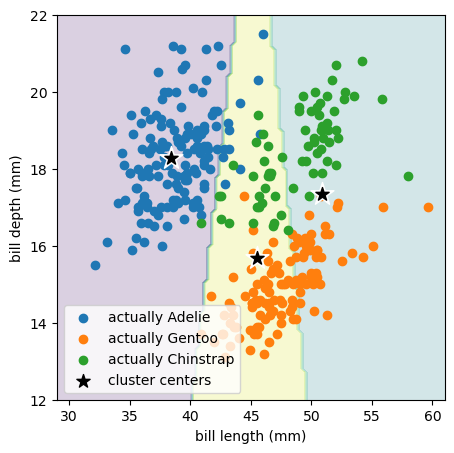
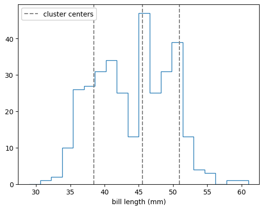
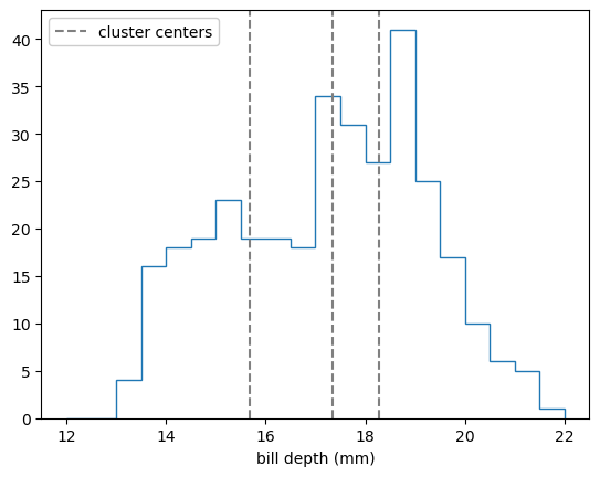
Remember that the k-means algorithm only sees the bill length and bill depth points without species labels (without colors in the above plot). It chose to place the 3 cluster centers in a way that’s mostly spaced by bill length (horizontally) because the raw distribution is more clumpy in bill length than bill depth:

fig, ax = plt.subplots()

ax.hist(features[:, 0], bins=20, range=(29, 61), histtype="step")
ax.set_xlabel("bill length (mm)")

for x, y in best_fit.cluster_centers_:
    label = ax.axvline(x, color="gray", ls="--")

ax.legend([label], ["cluster centers"], loc="upper left", framealpha=1)

plt.show()

fig, ax = plt.subplots()

ax.hist(features[:, 1], bins=20, range=(12, 22), histtype="step")
ax.set_xlabel("bill depth (mm)")

for x, y in best_fit.cluster_centers_:
    label = ax.axvline(y, color="gray", ls="--")

ax.legend([label], ["cluster centers"], loc="upper left", framealpha=1)

plt.show()

With more clusters, we can more identify more of its structure:

best_fit = KMeans(8).fit(features)

fig, ax = plt.subplots(figsize=(5, 5))

plot_clusters(best_fit)
plot_points(features, hidden_truth)

ax.scatter(*best_fit.cluster_centers_.T, color="white", marker="*", s=300)
ax.scatter(*best_fit.cluster_centers_.T, color="black", marker="*", s=100, label="cluster centers")

ax.legend(loc="lower left")

plt.show()

But now we’re subdividing clumps of data that we might want to keep together.

We can continue all the way from \(k = 1\) (all points in a single cluster) to \(k = n\) (every point in its own cluster) with this general trade-off: small \(k\) can ignore structure and large \(k\) can invent structure. There is a goodness-of-fit measure for this, explained variance, which compares the variance of cluster centers to the variance of points in each cluster: good clustering has small variance in each cluster. However, this can’t be used to choose \(k\), since it’s optimal for \(k = n\) (when every point is its own cluster, its variance is \(0\)).

Gaussian mixture models

One of the assumptions built into k-means fitting is that points should belong to the cluster center that is closest to it in all dimensions equally. Thus, the area that belongs to each cluster is roughly circular (Voronoi tiles, which is how soap bubbles fill a space). We can generalize the k-means algorithm a little bit by replacing each cluster center with a Gaussian ellipsoid. Instead of a boolean membership like \(\vec{x}_i \in C_j\), we can associate each \(\vec{x}_i\) to all the clusters by varying degrees:

\[\mbox{membership}_{C_j}(\vec{x}_i) \propto \mbox{Gaussian}(\vec{x}_i; \vec{\mu}_j, \hat{\sigma}_j)\]

That is, a point \(\vec{x}_i\) would mostly belong to a cluster \(C_j\) if it’s within fewer standard deviations of the cluster’s mean \(\vec{\mu}_j\), scaled by its covariance matrix \(\hat{\sigma}_j\), than other clusters \(C_{j'}\) (\(j' \ne j\)). However, each point is a member of all clusters to different degrees, and some points may be on a boundary, where the degree of their membership in two clusters is about equal. We can turn this “soft clustering” into a “hard clustering” like k-means by considering only the maximum \(\mbox{membership}_{C_j}(\vec{x}_i)\) for each point.

What’s more important is that the covariance matrices allow the clusters to extend in long strips if necessary.

from sklearn.mixture import GaussianMixture

best_fit = GaussianMixture(3).fit(features)

This model has 3 mean vectors (\(\vec{\mu}_j\)):

best_fit.means_

array([[49.24026349, 17.93788547],
       [38.84013815, 18.28259254],
       [47.01326276, 14.73564259]])

and 3 covariance matrices (\(\hat{\sigma}_j\)):

best_fit.covariances_

array([[[11.14282381,  1.14489971],
        [ 1.14489971,  2.27814016]],

       [[ 6.90219129,  0.91680438],
        [ 0.91680438,  1.44872906]],

       [[ 6.9000992 ,  1.43338999],
        [ 1.43338999,  0.67353676]]])

fig, ax = plt.subplots(figsize=(5, 5))

plot_clusters(best_fit)
plot_points(features, hidden_truth)

ax.scatter(*best_fit.means_.T, color="white", marker="*", s=300)
ax.scatter(*best_fit.means_.T, color="black", marker="*", s=100, label="cluster centers")

ax.legend(loc="lower left")

plt.show()

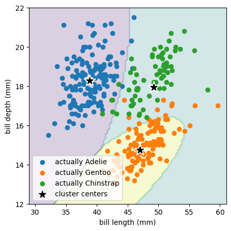
This Gaussian mixture model is more effective at discovering the true penguin species because the species’ distributions are not round in bill length and bill depth, but somewhat more ellipsoidal.

Now imagine that penguins in the antarctic don’t come labeled with species names (which is true). What compels us to invent these labels and put real things (the live penguins) into these imaginary categories (the species)? I would say it’s because we see patterns of density and sparsity in their distributions of attributes. Clustering formalizes this idea, including the ambiguity in the number of clusters and the points at the edges between clusters. All categories in nature larger than the fundamental particles are formed by some kind of clustering, formal or informal.

Hierarchical clustering

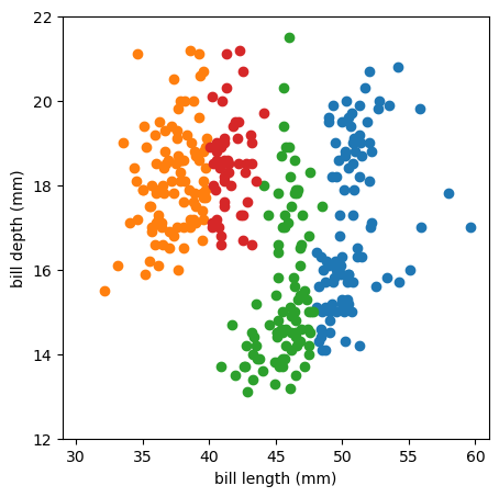
Instead of specifying the number of clusters, we could have specified a cut-off threshold: penguins are considered distinct if their distance in bill length, bill depth space is larger than some number of millimeters. This is called hierarchical or agglomerative clustering.

from sklearn.cluster import AgglomerativeClustering

best_fit = AgglomerativeClustering(n_clusters=None, distance_threshold=30).fit(features)

This algorithm doesn’t have a predict method, since it’s a recursive algorithm in which adding a point to a cluster would change how additional points are added to the cluster, but we can get the cluster assignments for the input data.

best_fit.labels_

array([1, 1, 3, 1, 1, 1, 1, 3, 1, 1, 1, 1, 3, 1, 2, 1, 1, 1, 1, 1, 1, 3,
       3, 1, 3, 1, 1, 1, 3, 1, 1, 1, 3, 1, 1, 1, 3, 1, 3, 1, 1, 3, 1, 3,
       1, 3, 1, 3, 1, 3, 1, 3, 1, 1, 1, 3, 1, 3, 1, 3, 1, 3, 1, 3, 1, 1,
       1, 2, 1, 3, 3, 1, 1, 3, 1, 3, 1, 1, 1, 3, 1, 1, 1, 1, 1, 3, 1, 1,
       1, 3, 1, 3, 1, 3, 1, 3, 1, 1, 1, 1, 1, 1, 1, 3, 1, 2, 1, 3, 1, 3,
       1, 1, 1, 3, 1, 1, 3, 3, 1, 3, 1, 3, 1, 2, 1, 3, 1, 1, 1, 3, 1, 3,
       1, 1, 3, 3, 1, 3, 1, 1, 1, 1, 1, 1, 1, 3, 2, 0, 0, 0, 2, 2, 2, 2,
       2, 2, 2, 0, 2, 0, 2, 0, 2, 0, 2, 0, 0, 2, 2, 2, 2, 2, 2, 0, 0, 2,
       2, 2, 0, 0, 0, 2, 2, 2, 0, 2, 0, 2, 0, 0, 2, 2, 0, 2, 2, 2, 0, 2,
       0, 2, 2, 2, 2, 2, 0, 2, 2, 2, 0, 2, 0, 0, 2, 0, 2, 2, 0, 2, 2, 0,
       2, 0, 2, 2, 0, 0, 2, 0, 2, 0, 2, 0, 2, 0, 2, 0, 2, 0, 2, 0, 0, 2,
       0, 0, 0, 0, 2, 0, 2, 2, 0, 2, 0, 0, 0, 2, 0, 2, 0, 0, 2, 2, 0, 2,
       0, 2, 0, 0, 2, 0, 2, 2, 0, 2, 0, 2, 0, 2, 0, 2, 0, 0, 0, 2, 0, 3,
       2, 3, 0, 2, 0, 0, 0, 2, 0, 3, 0, 3, 0, 0, 2, 2, 0, 2, 0, 0, 2, 0,
       2, 0, 0, 0, 0, 0, 0, 0, 0, 2, 0, 3, 0, 2, 0, 0, 2, 0, 2, 2, 0, 3,
       0, 0, 0])

A distance threshold of \(\mbox{30 mm}\) results in

len(np.unique(best_fit.labels_))

4

unique clusters. Here’s a plot:

fig, ax = plt.subplots(figsize=(5, 5))

for label in np.unique(best_fit.labels_):
    ax.scatter(*features[best_fit.labels_ == label].T)

ax.set_xlim(29, 61)
ax.set_ylim(12, 22)
ax.set_xlabel("bill length (mm)")
ax.set_ylabel("bill depth (mm)")

plt.show()

For this algorithm, you have to specify two kinds of distance metrics:

• a metric for the distance between two points, \(\vec{x}_{i}\) and \(\vec{x}_{i'}\) (\(i' \ne i\)), which could be Euclidean, but there are other choices (also affected by the choice of coordinates),

• a “linkage,” which specifies the distance between two clusters, \(C_j\) and \(C_{j'}\). Clusters are made of points, so the linkage is how pointwise distances are combined into a cluster distance. Some examples:

  • single: the distance between \(C_j\) and \(C_{j'}\) is the minimum distance between any \(\vec{x}_i\) in \(C_j\) and any \(\vec{x}_{i'}\) in \(C_{j'}\). Single linkage tends to make long, snakey clusters.

  • complete: the distance between \(C_j\) and \(C_{j'}\) is the maximum distance between any \(\vec{x}_i\) in \(C_j\) and any \(\vec{x}_{i'}\) in \(C_{j'}\). Complete linkage tends to make circular clusters in a Euclidean metric and the equivalent in other metrics (Manhattan/taxicab metric makes diamonds, Chebyshev metric makes squares, etc.).

  • average: the distance between two clusters is the average distance between all their pairs of points or between the cluster centers.

  • Wald: minimizes the variance within a cluster (used by default by Scikit-Learn, above).

Adding a point to a cluster changes the shape of the cluster, which affects how all subsequent points are added to clusters. This algorithm starts by considering each point as a separate cluster, then merging nearby clusters before more distant clusters, reevaluating all distances as the clusters change shape.

I’m mentioning this algorithm because it is important for HEP: jet-finding is an implementation of hierarchical clustering with HEP-specific choices for the measures above. In the FastJet manual (ref), you’ll find that the distance between two particle momenta \(i\) and \(i'\) in the anti-kT algorithm is

\[d_{ii'} = \mbox{min}\left(\left(\frac{1}{p_{Ti}}\right)^2, \left(\frac{1}{p_{Ti'}}\right)^2\right) \frac{(\eta_i - \eta_{i'})^2 + (\phi_i - \phi_{i'})^2}{(\Delta R)^2}\]

where \(p_{Ti}\), \(\eta_i\), and \(\phi_i\) are the transverse momentum, pseudorapidity, and azimuthal angle of particle \(i\), respectively, and similarly for \(i'\). The \(\Delta R\) parameter is a user-chosen jet scale cut-off. This is a Euclidean metric in \(\eta\)-\(\phi\) (which is uniformly populated by QCD backgrounds in hadron collisions).

The linkage is similar to the “average” above: to find the distance between two partial clusters, called “pseudojets,” you compute the vector-sum of the momenta of all particles in the pseudojet to get just one momentum, and then compare pseudojets in the same way you’d compare particles. Weighting the distances by the inverse transverse momentum squared prevents clusters from changing radically as they grow: we like the anti-kT algorithm because it’s stable, even when jets are surrounded by low-energy noise.

One more complication: HEP jet-finding algorithms also include a special “beam jet” whose distance from particle \(i\) is

\[d_{iB} = \left(\frac{1}{p_{Ti}}\right)^2\]

and it is usually ignored, so that the remaining jets are far from the QCD background that is expected along the beamline.

Apart from these choices, HEP jet-finding is standard hierarchical clustering.

Neural networks

So far, all of the clustering algorithms that I’ve shown are not neural networks. Deep learning approaches to the same problem are covered in the next section.