Solutions (NO PEEKING!)#
Do not look at this section until you have attempted to solve the problem yourself.
import numpy as np
import pandas as pd
import matplotlib.pyplot as plt

import torch
from torch import nn, optim
from torch.utils.data import TensorDataset, DataLoader, random_split
expected_ROC = np.array([
    [0,               0.01886829927], [0.0001020304051, 0.1289489538],
    [0.0004081216202, 0.209922966  ], [0.0009182736455, 0.3068408332],
    [0.001632486481,  0.376408661  ], [0.002550760127,  0.4303733732],
    [0.003673094582,  0.4678969334 ], [0.004999489848,  0.5027722976],
    [0.006529945924,  0.526339701  ], [0.00826446281,   0.5538282184],
    [0.01020304051,   0.5764214002 ], [0.01234567901,   0.6020473392],
    [0.01469237833,   0.6217746216 ], [0.01724313846,   0.6441249222],
    [0.01999795939,   0.6616243646 ], [0.02295684114,   0.6776505449],
    [0.0261197837,    0.6922878624 ], [0.02948678706,   0.7049561472],
    [0.03305785124,   0.7174712901 ], [0.03683297623,   0.7281837347],
    [0.04081216202,   0.7378146857 ], [0.04499540863,   0.7487390868],
    [0.04938271605,   0.7581570351 ], [0.05397408428,   0.7678773984],
    [0.05876951331,   0.7770101384 ], [0.06376900316,   0.7856509131],
    [0.06897255382,   0.7942924103 ], [0.07438016529,   0.8015956393],
    [0.07999183757,   0.8080126115 ], [0.08580757066,   0.8131647638],
    [0.09182736455,   0.8193828345 ], [0.09805121926,   0.8250768418],
    [0.1044791348,    0.8305736234 ], [0.1111111111,    0.8350616401],
    [0.1179471483,    0.8392843805 ], [0.1249872462,    0.843458635 ],
    [0.132231405,     0.8485805236 ], [0.1396796245,    0.8527170936],
    [0.1473319049,    0.8568358996 ], [0.1551882461,    0.8609808587],
    [0.1632486481,    0.8650308152 ], [0.1715131109,    0.8690270267],
    [0.1799816345,    0.8728376092 ], [0.188654219,     0.8768071621],
    [0.1975308642,    0.8809618493 ], [0.2066115702,    0.8844406165],
    [0.2158963371,    0.8878818684 ], [0.2253851648,    0.8913015608],
    [0.2350780533,    0.895321326  ], [0.2449750026,    0.8988141059],
    [0.2550760127,    0.9023606647 ], [0.2653810836,    0.9060166576],
    [0.2758902153,    0.9095274507 ], [0.2866034078,    0.9131203545],
    [0.2975206612,    0.9160367475 ], [0.3086419753,    0.9194866744],
    [0.3199673503,    0.9227445269 ], [0.331496786,     0.9258525464],
    [0.3432302826,    0.9288425431 ], [0.35516784,      0.9320369642],
    [0.3673094582,    0.934770168  ], [0.3796551372,    0.937793916 ],
    [0.3922048771,    0.9407399938 ], [0.4049586777,    0.9435231388],
    [0.4179165391,    0.946281785  ], [0.4310784614,    0.9488092479],
    [0.4444444444,    0.9518475898 ], [0.4580144883,    0.9547152601],
    [0.471788593,     0.9572437037 ], [0.4857667585,    0.959630249 ],
    [0.4999489848,    0.9625112252 ], [0.5143352719,    0.9647093883],
    [0.5289256198,    0.9668044304 ], [0.5437200286,    0.9689679766],
    [0.5587184981,    0.9712781888 ], [0.5739210285,    0.9728035781],
    [0.5893276196,    0.9748502201 ], [0.6049382716,    0.9769168758],
    [0.6207529844,    0.9783125007 ], [0.636771758,     0.9804721129],
    [0.6529945924,    0.982129956  ], [0.6694214876,    0.9841034064],
    [0.6860524436,    0.9858651034 ], [0.7028874605,    0.9875667363],
    [0.7199265381,    0.9892142364 ], [0.7371696766,    0.9907125562],
    [0.7546168758,    0.9919437219 ], [0.7722681359,    0.9932740291],
    [0.7901234568,    0.9942632436 ], [0.8081828385,    0.9954980595],
    [0.826446281,     0.9962563498 ], [0.8449137843,    0.9970929737],
    [0.8635853484,    0.9977009724 ], [0.8824609734,    0.9984200208],
    [0.9015406591,    0.9988781108 ], [0.9208244057,    0.9991514607],
    [0.940312213,     0.9994587815 ], [0.9600040812,    0.999709012 ],
    [0.9799000102,    0.9998581822 ], [1,               1           ],
])
Step 1: download and understand the data#
hls4ml_lhc_jets_hlf = pd.read_parquet("data/hls4ml_lhc_jets_hlf.parquet")
features = hls4ml_lhc_jets_hlf.drop("jet_type", axis=1)
targets = hls4ml_lhc_jets_hlf["jet_type"]
Step 2: split the data into training, validation, and test samples#
dataset = torch.utils.data.TensorDataset(
    torch.tensor(features.values, dtype=torch.float32),
    torch.tensor(targets.cat.codes.values, dtype=torch.int64),
)
subset_train, subset_valid, subset_test = torch.utils.data.random_split(dataset, [0.8, 0.1, 0.1])
Step 3: build a classifier neural network#
Not all of the features are close to the interval \((-1, 1)\), so you needed to scale each column to have zero mean and unit standard deviation.
Since this is a machine-optimized part of the fit, let’s use only the training sample to determine the mean and standard deviation of each feature.
class ScaleInputs(nn.Module):
    def __init__(self, subset_train):
        super().__init__()

        # get a single features tensor for the whole training subset
        ((features_tensor, targets_tensor),) = DataLoader(subset_train, batch_size=len(targets))

        # get 16 means and 16 standard deviations from the training dataset
        self.register_buffer("means", features_tensor.mean(axis=0))
        self.register_buffer("stds", features_tensor.std(axis=0))

    def forward(self, x):
        return (x - self.means) / self.stds
scale_inputs = ScaleInputs(subset_train)
model_without_softmax = nn.Sequential(
    scale_inputs,
    nn.Linear(16, 32),   # 16 input features → a hidden layer with 32 neurons
    nn.ReLU(),           # ReLU avoids the vanishing gradients problem
    nn.Linear(32, 32),   # first hidden layer → second hidden layer
    nn.ReLU(),
    nn.Linear(32, 32),   # second hidden layer → third hidden layer
    nn.ReLU(),
    nn.Linear(32, 5),    # third hidden layer → 5 output category probabilities
    # no softmax because CrossEntropyLoss automatically applies it
)
Step 4: monitor the loss function#
The following fits the model with loss function monitoring integrated into the loop.
NUM_EPOCHS = 10
BATCH_SIZE = 20000

# DataLoader lets us iterate over mini-batches, given a Subset
train_loader = DataLoader(subset_train, batch_size=BATCH_SIZE)
# the validation sample doesn't need to be batched, so we make it one big batch
valid_loader = DataLoader(subset_valid, batch_size=len(subset_valid))

loss_function = nn.CrossEntropyLoss()

optimizer = optim.Adam(model_without_softmax.parameters(), lr=0.03)

# collect loss data versus epoch
valid_loss_vs_epoch = []
train_loss_vs_epoch = []

for epoch in range(NUM_EPOCHS):
    # this asserts that the validation_loader iterates over exactly one batch
    ((features_tensor, targets_tensor),) = valid_loader

    predictions_tensor = model_without_softmax(features_tensor)
    loss = loss_function(predictions_tensor, targets_tensor)
    valid_loss = loss.item() * len(targets_tensor) * (0.8 / 0.1)  # normalize!

    valid_loss_vs_epoch.append(valid_loss)

    # the training sample needs a mini-batch loop
    train_loss = 0
    for features_tensor, targets_tensor in train_loader:
        optimizer.zero_grad()

        predictions_tensor = model_without_softmax(features_tensor)
        loss = loss_function(predictions_tensor, targets_tensor)
        train_loss += loss.item() * len(targets_tensor)           # normalize!

        loss.backward()
        optimizer.step()

    train_loss_vs_epoch.append(train_loss)

    # print out partial quantities so we can discover mistakes early
    print(f"{epoch = } {train_loss = } {valid_loss = }")
epoch = 0 train_loss = 656337.8393650055 valid_loss = 1071707.215309143
epoch = 1 train_loss = 518766.725063324 valid_loss = 540377.5119781494
epoch = 2 train_loss = 517470.5491065979 valid_loss = 505726.83095932007
epoch = 3 train_loss = 487575.9651660919 valid_loss = 503334.80739593506
epoch = 4 train_loss = 468018.2754993439 valid_loss = 478513.2737159729
epoch = 5 train_loss = 461054.63314056396 valid_loss = 466725.7137298584
epoch = 6 train_loss = 455747.1492290497 valid_loss = 460224.7953414917
epoch = 7 train_loss = 451280.24315834045 valid_loss = 455538.227558136
epoch = 8 train_loss = 447718.0783748627 valid_loss = 450266.42751693726
epoch = 9 train_loss = 446533.06698799133 valid_loss = 447064.2924308777
fig, ax = plt.subplots()

ax.plot(range(len(train_loss_vs_epoch)), train_loss_vs_epoch, marker=".")
ax.plot(range(len(valid_loss_vs_epoch)), valid_loss_vs_epoch, marker=".")

ax.grid(True, "both", "y", linestyle=":")

ax.set_xticks(range(NUM_EPOCHS))
ax.set_ylim(0, 1.2*max(max(train_loss_vs_epoch), max(valid_loss_vs_epoch)))
ax.set_xlabel("epoch number")
ax.set_ylabel("loss")
ax.legend(["training sample", "validation sample"])

plt.show()
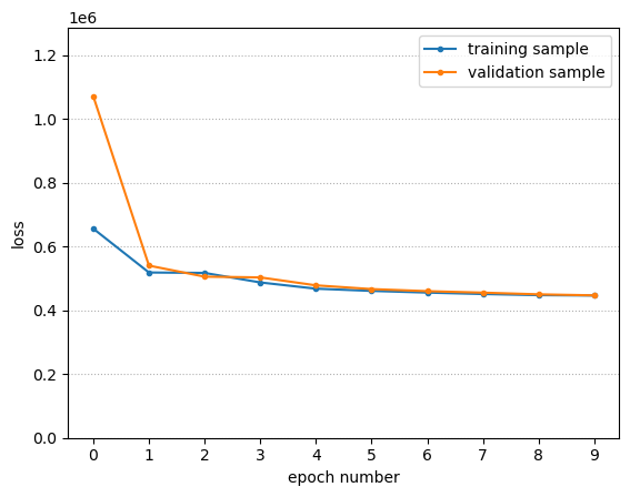
With smaller BATCH_SIZE, it converges to the same final loss in a smaller number of epochs (less total time).
To make the above plot interesting, BATCH_SIZE was chosen larger than it needed to be!
I see no sign of overfitting. This dataset has a lot of data points and they are not degenerate (all laying in a line/plane/hyperplane) and the neural network is not too large for it. There’s no need to add any regularization.
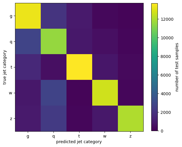
Step 5: compute a 5×5 confusion matrix#
To compute predictions as probabilities, we’ll need to apply the softmax function, so make a new model that has this included.
model_with_softmax = nn.Sequential(
    model_without_softmax,
    nn.Softmax(dim=1),
)
The first time you make this plot, it should use the validation sample (valid_loader).
Below, I’m using the test sample (test_loader) because I’ve already checked the validation sample and I won’t be making any more changes to my model or fitting procedure.
test_loader = DataLoader(subset_test, batch_size=len(subset_test))

((features_tensor, targets_tensor),) = test_loader
predictions_tensor = model_with_softmax(features_tensor)

confusion_matrix = np.array(
    [
        [
            (predictions_tensor[targets_tensor == true_class].argmax(axis=1) == prediction_class).sum().item()
            for prediction_class in range(5)
        ]
        for true_class in range(5)
    ]
)
confusion_matrix
array([[13248,  2046,   986,   280,   184],
       [ 2798, 11511,   893,   552,   258],
       [ 1602,   575, 13674,   831,   360],
       [  879,  2740,   166, 12700,   228],
       [  972,  2333,   232,   908, 12044]])
A colorbar plot demonstrates the quality of this model: the diagonal (correct predictions) is much more populated than the off-diagonals.
fig, ax = plt.subplots(figsize=(7, 7))

image = ax.imshow(confusion_matrix, vmin=0)
fig.colorbar(image, ax=ax, label="number of test samples", shrink=0.8)

ax.set_xticks(range(5), targets.cat.categories)
ax.set_yticks(range(5), targets.cat.categories)

ax.set_xlabel("predicted jet category")
ax.set_ylabel("true jet category")

None
Step 6: project it down to a 2×2 confusion matrix#
The following selects true heavy/electroweak events using is_heavy and determines if the model predicts heavy/electroweak if the sum of the 't', 'w', 'z' probabilities is greater than the threshold.
It would have been entirely equivalent to define a true light/QCD selection as
is_light = (targets_tensor < 2)
and a light/QCD prediction as
selected_predictions[:, 0:2].sum(axis=1) <= threshold
Each (length-5) row vector in the predictions consists of non-overlapping probabilities that add up to 1 (by construction, because of the softmax). So the sum of slice 0:2 is equal to 1 minus the sum of slice 2:5.
def matrix_for_cutoff_decision_at(threshold):
    is_heavy = (targets_tensor >= 2)

    true_positive  = (predictions_tensor[is_heavy][:, 2:5].sum(axis=1) > threshold).sum().item()
    false_positive = (predictions_tensor[~is_heavy][:, 2:5].sum(axis=1) > threshold).sum().item()

    false_negative = (predictions_tensor[is_heavy][:, 2:5].sum(axis=1) <= threshold).sum().item()
    true_negative  = (predictions_tensor[~is_heavy][:, 2:5].sum(axis=1) <= threshold).sum().item()

    return np.array([
        [true_positive, false_positive],
        [false_negative, true_negative],
    ])
matrix_for_cutoff_decision_at(0.5)
array([[41167,  3116],
       [ 9077, 29640]])
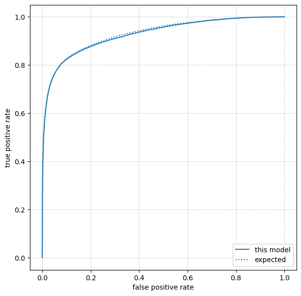
Step 7: plot a ROC curve#
Once we have 2×2 confusion matrices as a function of threshold, we can plot the ROC curve as in the section on Goodness of fit metrics.
true_positive_rates = []
false_positive_rates = []

for threshold in np.linspace(0, 1, 1000):
    ((true_positive, false_positive),
     (false_negative, true_negative)) = matrix_for_cutoff_decision_at(threshold)

    true_positive_rates.append(true_positive / (true_positive + false_negative))
    false_positive_rates.append(false_positive / (true_negative + false_positive))
fig, ax = plt.subplots(figsize=(7, 7))

ax.plot(false_positive_rates, true_positive_rates, label="this model")
ax.plot(expected_ROC[:, 0], expected_ROC[:, 1], ls=":", color="tab:blue", label="expected")

ax.grid(True, linestyle=":")

ax.set_xlabel("false positive rate")
ax.set_ylabel("true positive rate")

ax.legend(loc="lower right")

plt.show()