End-to-End Scikit-HEP Analysis Pipeline

In the previous chapters you met uproot, awkward, vector, and hist one at a time. This chapter chains them into a single, realistic analysis: we will look for evidence of the Higgs boson in the $H \rightarrow ZZ^* \rightarrow 4\ell$ channel, using ATLAS Open Data from the 2015 and 2016 proton-proton runs.

The data is read in chunks, so the notebook runs in a small, fixed amount of memory however many files you process.

Reading the data¶

We use the 4lep skim of the ATLAS Run 2 open data: 16 files, 660 MB in total, holding 1.5 million events that contain at least four leptons. The files are plain ROOT ntuples, so uproot can read them directly.

Only eight branches are needed, and we read them a chunk at a time rather than all at once, so memory use stays flat no matter how much data is enabled below.

import awkward as ak
import hist
import matplotlib.pyplot as plt
import uproot
import vector
from hepunits import GeV, MeV
from particle import Particle

vector.register_awkward()

# Particle stores masses in MeV; hepunits does the conversion for us.
MZ = Particle.from_pdgid(23).mass * MeV / GeV

# By default each file is downloaded whole over HTTPS into a temporary
# directory, which takes about a minute for the whole dataset and works
# everywhere, Windows included. Note that reading over plain HTTPS without that
# cache does not work: opendata.cern.ch rate-limits (HTTP 429) the many small
# range requests uproot would otherwise make.
#
# If you have XRootD, set USE_XROOTD = True to stream only the branches we ask
# for instead of downloading whole files.
USE_XROOTD = False

if USE_XROOTD:
    BASE = "root://eospublic.cern.ch//eos/opendata/atlas/rucio/opendata"
else:
    BASE = "simplecache::https://opendata.cern.ch/eos/opendata/atlas/rucio/opendata"

# All 16 files: 660 MB, 1.5M events, about a minute to process. Comment some
# out for a quicker run, at the cost of a much less convincing peak.
PERIODS = [
    "data16_periodL",
    "data16_periodI",
    "data16_periodD",
    "data16_periodG",
    "data16_periodF",
    "data16_periodC",
    "data16_periodK",
    "data15_periodJ",
    "data16_periodB",
    "data16_periodE",
    "data15_periodG",
    "data16_periodA",
    "data15_periodE",
    "data15_periodF",
    "data15_periodH",
    "data15_periodD",
]
FILES = [f"{BASE}/ODEO_FEB2025_v0_4lep_{p}.4lep.root" for p in PERIODS]

BRANCHES = [
    "lep_pt", "lep_eta", "lep_phi", "lep_e",
    "lep_charge", "lep_type", "lep_isTightID", "lep_isTightIso",
]

# These branches come to about 225 bytes per event, so 25 MiB is roughly
# 117k events per chunk.
STEP_SIZE = "25 MiB"

The analysis logic¶

Picking any four leptons and adding up their four-momenta does not work. Three things have to be right, and each one is a cut that matters enormously:

Lepton quality. The skim is deliberately loose, applying no quality requirements at all. Without lep_isTightID and lep_isTightIso, roughly 424,000 “candidates” survive and about 18,000 land in the Higgs mass window — some 500 times the real signal, almost all of it misidentified jets. With the cuts applied, 911 events remain.

The second Z is off-shell. Since $m_H = 125\ \text{GeV}$ is below $2m_Z = 182\ \text{GeV}$ , the Higgs cannot decay into two on-shell Z bosons. One is real and the other is virtual ( $Z^*$ ), typically well below 91 GeV. This is why the two mass windows below are deliberately asymmetric: demanding that both pairs sit near the Z mass would throw away essentially all of the signal.

The two Z candidates must not share a lepton. ak.combinations over a list of lepton pairs will happily return two pairs built from overlapping leptons, and adding those four-momenta double-counts a lepton. On this dataset about 90% of the naive combinations are of that kind. The fix is ak.argcombinations, which gives the indices of the paired leptons rather than the leptons themselves, so we can require all four indices to be distinct.

def four_lepton_mass(events):
    """Return the m_4l of the best 4-lepton candidate in each event."""
    leptons = ak.zip(
        {
            "pt": events.lep_pt,
            "eta": events.lep_eta,
            "phi": events.lep_phi,
            "E": events.lep_e,
            "charge": events.lep_charge,
            "flavour": events.lep_type,  # 11 = electron, 13 = muon
            "tight_id": events.lep_isTightID,
            "tight_iso": events.lep_isTightIso,
        },
        with_name="Momentum4D",
    )

    # 1. Keep good leptons, then require exactly four of them with zero total
    #    charge. Note that the counting happens *after* the quality cuts.
    leptons = leptons[(leptons.pt > 5) & leptons.tight_id & leptons.tight_iso]
    leptons = leptons[
        (ak.num(leptons) == 4) & (ak.sum(leptons.charge, axis=1) == 0)
    ]

    # 2. Z candidates: opposite-charge, same-flavour pairs. argcombinations
    #    keeps the lepton indices, which step 3 needs.
    pairs = ak.argcombinations(leptons, 2, fields=["i", "j"])
    pairs = pairs[
        (leptons[pairs.i].charge != leptons[pairs.j].charge)
        & (leptons[pairs.i].flavour == leptons[pairs.j].flavour)
    ]

    # 3. Higgs candidates: pairs of Z candidates whose four leptons are all
    #    distinct, so that no lepton is counted twice.
    quads = ak.combinations(pairs, 2, fields=["za", "zb"])
    za, zb = quads.za, quads.zb
    quads = quads[
        (za.i != zb.i) & (za.i != zb.j) & (za.j != zb.i) & (za.j != zb.j)
    ]
    za, zb = quads.za, quads.zb

    # 4. Call the pair closer to the Z mass Z1 and the other Z2, then apply
    #    asymmetric windows: Z2 is the off-shell one, so it is allowed to be
    #    much lighter.
    mass_a = (leptons[za.i] + leptons[za.j]).mass
    mass_b = (leptons[zb.i] + leptons[zb.j]).mass
    a_is_leading = abs(mass_a - MZ) < abs(mass_b - MZ)

    m_z1 = ak.where(a_is_leading, mass_a, mass_b)
    m_z2 = ak.where(a_is_leading, mass_b, mass_a)

    keep = (m_z1 > 50) & (m_z1 < 106) & (m_z2 > 12) & (m_z2 < 115)
    quads, m_z1 = quads[keep], m_z1[keep]

    # 5. An event may still have several valid candidates; keep the one whose
    #    Z1 is closest to the Z mass.
    best = ak.argmin(abs(m_z1 - MZ), axis=1, keepdims=True)
    quads = quads[best]

    za, zb = quads.za, quads.zb
    m4l = leptons[za.i] + leptons[za.j] + leptons[zb.i] + leptons[zb.j]

    # keepdims=True above leaves missing values behind, hence drop_none.
    return ak.drop_none(ak.flatten(m4l.mass))

Processing the data and plotting¶

Now we loop over the files, read each one in chunks with TTree.iterate, and fill a hist histogram as we go. Only one chunk is ever in memory, so this would work just as well on a dataset far too large to load at once.

h = hist.Hist.new.Reg(29, 80, 250, name="m4l", label=r"$m_{4\ell}$ [GeV]").Double()

n_events = n_candidates = 0
masses = []  # kept for the fit further down

for path in FILES:
    with uproot.open(path) as file:
        for chunk in file["analysis"].iterate(BRANCHES, step_size=STEP_SIZE):
            m4l = four_lepton_mass(chunk)
            h.fill(m4l)
            masses.append(m4l)

            n_events += len(chunk)
            n_candidates += len(m4l)

masses = ak.concatenate(masses)

print(f"events read: {n_events:,}")
print(f"total candidates: {n_candidates:,}")

for lo, hi, label in [
    (80, 100, "Z -> 4l"),
    (115, 130, "Higgs window"),
    (180, 250, "ZZ continuum"),
]:
    print(f"  {label:14s} {h[hist.loc(lo):hist.loc(hi)].sum():4.0f}")

fig, ax = plt.subplots(figsize=(9, 5))
h.plot(ax=ax, histtype="fill", color="#5B8FF9", edgecolor="black", linewidth=0.8)

ax.axvline(125, color="crimson", linestyle="--", linewidth=1.2)
ax.text(127, ax.get_ylim()[1] * 0.75, r"$m_H = 125$ GeV", color="crimson")

ax.set_ylabel("Candidates / bin")
ax.set_title(r"ATLAS Open Data 2015+2016: $H \to ZZ^* \to 4\ell$")
plt.show()

events read: 1,515,848
total candidates: 697
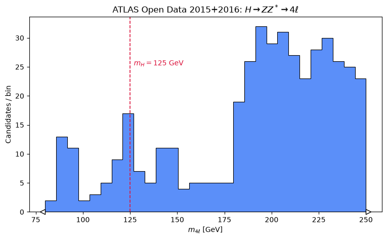
  Z -> 4l          26
  Higgs window     31
  ZZ continuum    319

What the plot shows¶

Three features are worth picking out, and only one of them is the Higgs:

A peak at 91 GeV. This is $Z \rightarrow 4\ell$ , a single Z boson decaying to four leptons through a virtual photon. It is a known, precisely measured process, which makes it a useful check: if the machinery can reconstruct this peak in the right place, it is probably assembling four-vectors correctly.
The ZZ continuum above 180 GeV. Once there is enough energy to produce two real Z bosons, the rate climbs steeply. This dominates the plot by sheer numbers.
An excess near 125 GeV, with about 31 candidates in the 115–130 GeV window over a background of roughly 15.

The peak looks sharper than it really is, though. The histogram uses 29 bins between 80 and 250 GeV, so each one is about 5.9 GeV wide, and the signal happens to fall almost entirely inside a single bin. Re-binned to 2.5 GeV the same events spread over two bins of roughly eight entries each, which is far less striking. Only the binning has changed, not the physics — worth remembering whenever a bump is judged by eye.

Comparing that excess against the sidebands gives a local significance of about $3.5\sigma$ . That is genuine evidence, and it is the right order of magnitude for this much data — but it is not a discovery. We have made no estimate of the systematic uncertainties, used a crude background model rather than simulation, and ignored the look-elsewhere effect. The real ATLAS measurement reached this level of sensitivity with the same data, and needed a great deal more care to turn it into a claim.

Fitting the peak¶

A bump that we can see is one thing; a number with an uncertainty is another. We can estimate the mass by fitting the region around the peak with a simple model: a Gaussian for the signal sitting on a flat background.

The fit is an extended unbinned maximum-likelihood fit, which uses the individual candidate masses rather than histogram bins — worth doing when there are only a handful of signal events, as there are here. iminuit provides both the likelihood (cost.ExtendedUnbinnedNLL) and the minimiser, so all we supply is a function returning the expected yield and the density.

import numpy as np
from iminuit import Minuit, cost
from scipy.stats import norm

FIT_LO, FIT_HI = 100.0, 160.0

candidates = ak.to_numpy(masses)
window = candidates[(candidates > FIT_LO) & (candidates < FIT_HI)]


def model(x, n_sig, n_bkg, m_higgs, resolution):
    """Expected yield and density: a Gaussian peak on a flat background."""
    peak = norm.pdf(x, m_higgs, resolution)
    peak /= norm.cdf(FIT_HI, m_higgs, resolution) - norm.cdf(
        FIT_LO, m_higgs, resolution
    )
    return n_sig + n_bkg, n_sig * peak + n_bkg / (FIT_HI - FIT_LO)


fit = Minuit(
    cost.ExtendedUnbinnedNLL(window, model),
    n_sig=20.0,
    n_bkg=len(window) - 20.0,
    m_higgs=125.0,
    resolution=2.5,
)
fit.limits["n_sig"] = (0, None)
fit.limits["n_bkg"] = (0, None)
fit.limits["m_higgs"] = (FIT_LO, FIT_HI)
fit.limits["resolution"] = (0.5, 10)
fit.migrad()
fit.hesse()

m_h, m_h_err = fit.values["m_higgs"], fit.errors["m_higgs"]
n_s, n_s_err = fit.values["n_sig"], fit.errors["n_sig"]

print(f"fit converged: {fit.valid}")
print(f"  m_H        = {m_h:.1f} +/- {m_h_err:.1f} GeV")
print(f"  resolution = {fit.values['resolution']:.1f}"
      f" +/- {fit.errors['resolution']:.1f} GeV")
print(f"  signal     = {n_s:.0f} +/- {n_s_err:.0f} events"
      f"  ({n_s / n_s_err:.1f} sigma)")
print(f"  background = {fit.values['n_bkg']:.0f}"
      f" +/- {fit.errors['n_bkg']:.0f} events")

bins = np.linspace(FIT_LO, FIT_HI, 25)
width = bins[1] - bins[0]
counts, _ = np.histogram(window, bins=bins)
centres = 0.5 * (bins[1:] + bins[:-1])

curve_x = np.linspace(FIT_LO, FIT_HI, 400)
_, curve_y = model(curve_x, *fit.values)

fig, ax = plt.subplots(figsize=(9, 5))
ax.errorbar(centres, counts, yerr=np.sqrt(counts), fmt="ko", label="ATLAS Open Data")
ax.plot(curve_x, curve_y * width, color="crimson", linewidth=2,
        label="signal + background")
ax.axhline(fit.values["n_bkg"] / (FIT_HI - FIT_LO) * width, color="#5B8FF9",
           linestyle="--", linewidth=1.5, label="background only")

ax.set_xlabel(r"$m_{4\ell}$ [GeV]")
ax.set_ylabel(f"Candidates / {width:.1f} GeV")
ax.set_title(rf"Fitted peak: $m_H = {m_h:.1f} \pm {m_h_err:.1f}$ GeV")
ax.legend(frameon=False)
plt.show()

fit converged: True
  m_H        = 123.4 +/- 1.4 GeV
  resolution = 3.3 +/- 0.9 GeV
  signal     = 16 +/- 6 events  (2.6 sigma)
  background = 62 +/- 9 events

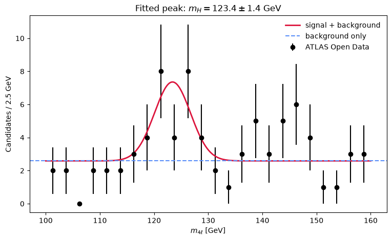
The fit returns a mass of about 123.4 GeV with an uncertainty of roughly 1.4 GeV, against the known value of 125.25 GeV — agreement to a little over one standard deviation, from fewer than twenty signal events. Repeating the fit over different ranges, anywhere from 95–165 GeV to 110–150 GeV, moves the result by less than 0.1 GeV, so it is not an artefact of where we drew the window.

The fitted width is also meaningful. At about 3.3 GeV it is far wider than the Higgs boson’s natural width of a few MeV, so what we are really measuring is the detector’s mass resolution for four leptons.

That uncertainty is statistical only. A real measurement would add systematic uncertainties — the lepton energy and momentum scales above all — and would model the background from simulation rather than assuming it is flat. With a signal of only $2.6\sigma$ in this fit, the honest summary is that the data is consistent with the known Higgs boson mass, not that we have measured it.