ROOT file structure and terminology
A ROOT file (ROOT TFile, uproot.ReadOnlyFile) is like a little filesystem containing nested directories (ROOT TDirectory, uproot
Any class instance (ROOT TObject, uproot.Model) can be stored in a directory, including types such as histograms (e.g. ROOT TH1, uproot
One of these classes, TTree (ROOT TTree, uproot.TTree), is a gateway to large datasets. A TTree is roughly like a Pandas DataFrame in that it represents a table of data. The columns are called TBranches (ROOT TBranch, uproot.TBranch), which can be nested (unlike Pandas), and the data can have any C++ type (unlike Pandas, which can store any Python type).
A TTree is often too large to fit in memory, and sometimes (rarely) even a single TBranch is too large to fit in memory. Each TBranch is therefore broken down into TBaskets (ROOT TBasket, uprootextend writes in the previous lesson.) TBaskets are the smallest unit that can be read from a TTree: if you want to read the first entry, you have to read the first TBasket.
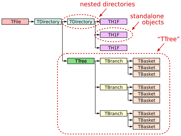
As a data analyst, you’ll likely be concerned with TTrees and TBranches first-hand, but only TBaskets when efficiency issues come up. Files with large TBaskets might require a lot of memory to read; files with small TBaskets will be slower to read (in ROOT also, but especially in Uproot). Megabyte-sized TBaskets are usually ideal.
import uproot

file_url = "root://eospublic.cern.ch//eos/opendata/cms/derived-data/AOD2NanoAODOutreachTool/Run2012BC_DoubleMuParked_Muons.root"

# If you are on Windows or don't have XRootD installed you can use this url instead
# file_url = "https://opendata.cern.ch/record/12341/files/Run2012BC_DoubleMuParked_Muons.root"

file = uproot.open(file_url)
file.classnames()
{'Events;75': 'TTree', 'Events;74': 'TTree'}Just asking for the uproot.TTree object and printing it out does not read the whole dataset.
tree = file["Events"]
tree.show()
name | typename | interpretation
---------------------+--------------------------+-------------------------------
nMuon | uint32_t | AsDtype('>u4')
Muon_pt | float[] | AsJagged(AsDtype('>f4'))
Muon_eta | float[] | AsJagged(AsDtype('>f4'))
Muon_phi | float[] | AsJagged(AsDtype('>f4'))
Muon_mass | float[] | AsJagged(AsDtype('>f4'))
Muon_charge | int32_t[] | AsJagged(AsDtype('>i4'))
Reading part of a TTree
In the last lesson, we learned that the most direct way to read one TBranch is to call uproot
# without entry_stop, it will take a long time and it might even fail
tree["nMuon"].array(entry_stop=10_000)However, it takes a long time because a lot of data have to be sent over the network.
To limit the amount of data read, set entry_start and entry_stop to the range you want. The entry_start is inclusive, entry_stop exclusive, and the first entry would be indexed by 0, just like slices in an array interface (first lesson). Uproot only reads as many TBaskets as are needed to provide these entries.
tree["nMuon"].array(entry_start=1_000, entry_stop=2_000)These are the building blocks of a parallel data reader: each is responsible for a different slice. (See also uprootentry_start/entry_stop in optimal ways.)
Reading multiple TBranches at once
Suppose you know that you will need all of the muon TBranches. Asking for them in one request is more efficient than asking for each TBranch individually because the server can be working on reading the later TBaskets from disk while the earlier TBaskets are being sent over the network to you. Whereas a TBranch has an array method, the TTree has an arrays (plural) method for getting multiple arrays.
muons = tree.arrays(
    ["Muon_pt", "Muon_eta", "Muon_phi", "Muon_mass", "Muon_charge"], entry_stop=1_000
)
muonsNow all five of these TBranches are in the output, muons, which is an Awkward Array. An Awkward Array of multiple TBranches has a dict-like interface, so we can get each variable from it by
muons["Muon_pt"]muons["Muon_eta"]muons["Muon_phi"] # etc.Selecting TBranches by name
Suppose you have many muon TBranches and you don’t want to list them all. The uproot.TTree.keys and uproot.TTree.arrays both take a filter_name argument that can select them in various ways (see documentation). In particular, it’s good to use the keys first, to know which branches match your filter, followed by arrays, to actually read them.
tree.keys(filter_name="Muon_*")['Muon_pt', 'Muon_eta', 'Muon_phi', 'Muon_mass', 'Muon_charge']tree.arrays(filter_name="Muon_*", entry_stop=1_000)(There are also filter_typename and filter_branch for more options.)
Scaling up, making a plot
The best way to figure out what you’re doing is to tinker with small datasets, and then scale them up. Here, we take 1000 events and compute dimuon masses.
muons = tree.arrays(entry_stop=1_000)
cut = muons["nMuon"] == 2

pt0 = muons["Muon_pt", cut, 0]
pt1 = muons["Muon_pt", cut, 1]
eta0 = muons["Muon_eta", cut, 0]
eta1 = muons["Muon_eta", cut, 1]
phi0 = muons["Muon_phi", cut, 0]
phi1 = muons["Muon_phi", cut, 1]

import numpy as np

mass = np.sqrt(2 * pt0 * pt1 * (np.cosh(eta0 - eta1) - np.cos(phi0 - phi1)))

import hist

masshist = hist.Hist(hist.axis.Regular(120, 0, 120, label="mass [GeV]"))
masshist.fill(mass)
masshist.plot();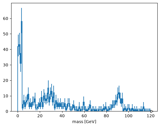
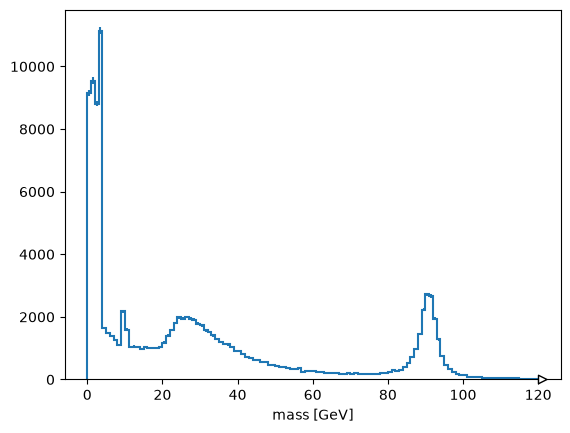
That worked (there’s a Z peak). Now to do this over the whole file, we should be more careful about what we’re reading,
tree.keys(filter_name=["nMuon", "/Muon_(pt|eta|phi)/"])['nMuon', 'Muon_pt', 'Muon_eta', 'Muon_phi']and accumulate data gradually with uprootentry_start/entry_stop in a loop.
masshist = hist.Hist(hist.axis.Regular(120, 0, 120, label="mass [GeV]"))

# You can remove the entry_stop, but it takes a long time
for muons in tree.iterate(filter_name=["nMuon", "/Muon_(pt|eta|phi)/"], step_size=50_000, entry_stop=250_000):
    cut = muons["nMuon"] == 2
    pt0 = muons["Muon_pt", cut, 0]
    pt1 = muons["Muon_pt", cut, 1]
    eta0 = muons["Muon_eta", cut, 0]
    eta1 = muons["Muon_eta", cut, 1]
    phi0 = muons["Muon_phi", cut, 0]
    phi1 = muons["Muon_phi", cut, 1]
    mass = np.sqrt(2 * pt0 * pt1 * (np.cosh(eta0 - eta1) - np.cos(phi0 - phi1)))
    masshist.fill(mass)
    print(masshist.sum() / tree.num_entries)

masshist.plot();
0.000401378521785351
0.0007917886413924456
0.0011923546889423702
0.0015963981262199199
0.001982485882894546
Getting data into NumPy or Pandas
In all of the above examples, the array, arrays, and iterate methods return Awkward Arrays. The Awkward Array library is useful for exactly this kind of data (jagged arrays: more in the next lesson), but you might be working with libraries that only recognize NumPy arrays or Pandas DataFrames.
Use library="np" or library="pd" to get NumPy or Pandas, respectively.
tree["nMuon"].array(library="np", entry_stop=10_000)array([2, 2, 1, ..., 2, 2, 2], shape=(10000,), dtype=uint32)tree.arrays(library="np", entry_stop=10_000){'nMuon': array([2, 2, 1, ..., 2, 2, 2], shape=(10000,), dtype=uint32),
'Muon_pt': array([array([10.763697, 15.736523], dtype=float32),
array([10.53849 , 16.327097], dtype=float32),
array([3.2753265], dtype=float32), ...,
array([30.238283, 13.035936], dtype=float32),
array([17.35597 , 15.874119], dtype=float32),
array([39.6421 , 42.273067], dtype=float32)],
shape=(10000,), dtype=object),
'Muon_eta': array([array([ 1.0668273, -0.5637865], dtype=float32),
array([-0.42778006, 0.34922507], dtype=float32),
array([2.2108555], dtype=float32), ...,
array([-1.1984524, -2.0278058], dtype=float32),
array([-0.83613676, -0.8279834 ], dtype=float32),
array([-2.090575 , -1.0396558], dtype=float32)],
shape=(10000,), dtype=object),
'Muon_phi': array([array([-0.03427272, 2.5426154 ], dtype=float32),
array([-0.2747921, 2.5397813], dtype=float32),
array([-1.2234136], dtype=float32), ...,
array([-2.2813563 , 0.60287297], dtype=float32),
array([-1.4231573, -1.4103615], dtype=float32),
array([ 2.2101276, -0.9990832], dtype=float32)],
shape=(10000,), dtype=object),
'Muon_mass': array([array([0.10565837, 0.10565837], dtype=float32),
array([0.10565837, 0.10565837], dtype=float32),
array([0.10565837], dtype=float32), ...,
array([0.10565837, 0.10565837], dtype=float32),
array([0.10565837, 0.10565837], dtype=float32),
array([0.10565837, 0.10565837], dtype=float32)],
shape=(10000,), dtype=object),
'Muon_charge': array([array([-1, -1], dtype=int32), array([ 1, -1], dtype=int32),
array([1], dtype=int32), ..., array([ 1, -1], dtype=int32),
array([ 1, -1], dtype=int32), array([ 1, -1], dtype=int32)],
shape=(10000,), dtype=object)}tree.arrays(library="pd", entry_stop=10_000)NumPy is great for non-jagged data like the "nMuon" branch, but it has to represent an unknown number of muons per event as an array of NumPy arrays (i.e. Python objects).
Pandas can be made to represent multiple particles per event by putting this structure in a pd.MultiIndex, but not when the DataFrame contains more than one particle type (e.g. muons and electrons). Use separate DataFrames for these cases. If it helps, note that there’s another route to DataFrames: by reading the data as an Awkward Array and calling ak.to_pandas on it. (Some methods use more memory than others, and I’ve found Pandas to be unusually memory-intensive.)
Or use Awkward Arrays (next lesson).