Introduction

Overview

Teaching: 10 min
Exercises: 0 min

Questions

• What is the purpose if this analysis?

Objectives

• Understand why we prepared this example analysis

• Understand what the analysis is doing

Why have we prepared this analysis?

We have prepared this example analysis as common baseline for learning the technologies discussed in this workshop. The goal is to have a working example that is simple yet complex enough to demonstrate common problems and their solutions in physics analysis.

The analysis is taken from the CERN Open Data portal and modified to fit our needs. You can find there additional information complementing the explanation below.

The analysis

This analysis uses data and simulated events at the CMS experiment from 2012 with the goal of studying decays of a Higgs boson into two tau leptons. The final state is a muon lepton and a hadronically decaying tau lepton. The analysis loosely follows the setup of the official CMS analysis published in 2014.

The purpose of the original CMS analysis was to establish the existence of the Higgs boson decaying into two tau leptons. Since performing this analysis properly with full consideration of all systematic uncertainties is an enormously complex task, we reduce this analysis to the qualitative study of the kinematics and properties of such events without a statistical analysis. However, as you can explore in this record, already such a reduced analysis is complex and requires extensive physics knowledge, which makes this a perfect first look into the procedures required to claim the evidence or existence of a new particle.

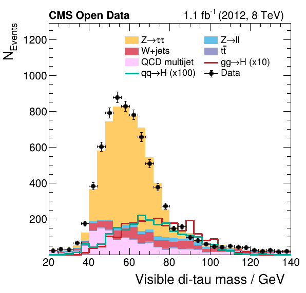
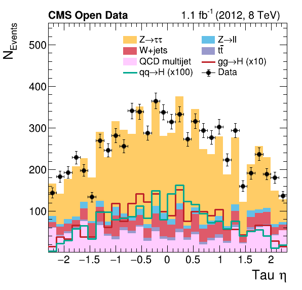
Two example results produced by this analysis can be seen below. The plots show the data recorded by the detector compared with the estimation of the contributing processes, which are explained below. The analysis has implemented the visualization of 34 such observables.

Analysis steps

The analysis steps follow the typical workflow of such an analysis at CMS. An overview of these steps is given in the following and the full details can be found in the analysis code and the description of the single sections of the lesson. The detailed technical description how to run the analysis is included separately in the respective section of the lesson.

1. First, the NanoAOD files containing data and simulated events are pre-processed. This step is called ‘skimming’ since the event selection reduces the size of the datasets significantly. In addition, we perform a pair selection to find from the muon and tau collections the pair which is most likely to have originated from the Higgs boson.
2. The first step produces skimmed datasets from the original files but still preserves information of selected quantities for each event. In this second step, we compute histograms of these quantities for all the skimmed datasets. Because of the data-driven QCD estimation (explained later in the physics background), similar histograms have to be produced with the selection containing same-charged tau lepton pairs. This sums up to multiple hundreds of histograms which have to be combined to produce the final plots such as the ones shown above.
3. Finally, the histograms are combined to produce the final plots showing the data taken with the CMS detector compared with the expectation from the background estimations. These plots make it possible to study the contribution of the different physics processes to the data taken with the CMS detector, and represent the first step towards verifying the existence of the Higgs boson.
4. To perform a measurement, we have to fit the expected contributions of physics processes to the data from the experiment. The procedure followed for this step is similar to what was done originally to measure the signal strength and claim the existence of the Higgs boson.

Disclaimer: How to interpret the results

Please note that a proper analysis of data always requires a thorough study of all uncertainties. Since this analysis does not include any systematic uncertainties, the resulting plots should be interpreted only qualitatively. For a valid physics measurement, the differences between the data and the sum of all processes would have to be explained within the uncertainties. Also note that the counts for the simulated Higgs boson events are scaled up to make the expected signal contribution visible by eye.

Reminder: Have you set up your environment?

Please go here, select one of the options to set up your environment with the required software and download the required files.

Key Points

• Example analysis used as common baseline for learning the technologies discussed at the workshop

• This analysis studies decays of a Higgs boson into two tau leptons in the final state of a muon lepton and a hadronically decayed tau lepton

Physics background

Overview

Teaching: 15 min
Exercises: 0 min

Questions

• What is the physics behind the data?

Objectives

• Learn the basics of the physics processes present in the data

The following sections describe the relevant physics processes of the analysis.

Signal process

The physical process of interest, also often called signal, is the production of the Higgs boson in the decay to two tau leptons. The main production modes of the Higgs boson are the gluon fusion and the vector boson fusion production indicated in the plots with the labels gg→H and qq→H, respectively. See below the two Feynman diagrams that describe the processes at leading order.

Tau decay modes

The tau lepton has a very short lifetime of about 290 femtoseconds after which it decays into other particles. With a probability of about 20% each, the tau lepton decays into a muon or an electron and two neutrinos. All other decay modes consist of a combination of hadrons such as pions and kaons and a single neutrino. You can find here a full overview and the exact numbers. This analysis considers only tau lepton pairs of which one tau lepton decays into a muon and two neutrinos and the other tau lepton hadronically, whereas the official CMS analysis considered additional decay channels.

Background processes

Besides the Higgs boson decaying into two tau leptons, many other processes can produce very similar signatures in the detector, which have to be taken into account to draw any conclusions from the data. In the following, the most prominent processes with a similar signature as the signal are presented. Besides the QCD multijet process, the analysis estimates the contribution of the background processes using simulated events.

Z→ττ

The most prominent background process is the Z boson decaying into two tau leptons. The leading order production is called the Drell-Yan process in which a quark anti-quark pair annihilates. Because the Z boson decays directly into two tau leptons, same as the Higgs boson, this process is very hard to distinguish from the signal.

Z→ll

Besides the decay of the Z boson into two tau leptons, the Z boson decays with the same probability to electrons and muons. Although this process does not contain any genuine tau leptons, a tau can be reconstructed by mistake. Objects that are likely to be misidentified as a hadronic decay of a tau lepton are electrons or jets.

W+jets

W bosons are frequently produced at the LHC and can decay into any lepton. If a muon from a W boson is selected together with a misidentified tau from a jet, a similar event signature as the signal can occur. However, this process can be strongly suppressed by a cut in the event selection on the transverse mass of the muon and the missing energy, as done in the published CMS analysis.

tt¯

Top anti-top pairs are produced at the LHC by quark anti-quark annihilation or gluon fusion. Because a top quark decays immediately and almost exclusively via a W boson and a bottom quark, additional misidentifications result in signal-like signatures in the detector similar to the $W+\mathrm{jets}$ process explained above. However, the identification of jets originating from bottom quarks, and the subsequent removel of such events, is capable of reducing this background effectively.

QCD

The QCD multijet background describes decays with a large number of jets, which occurs very often at the LHC. Such events can be falsely selected for the analysis due to misidentifications. Because a proper simulation of this process is complex and computational expensive, the contribution is not estimated from simulation but from data itself. Therefore, we select tau pairs with the same selection as the signal, but with the modified requirement that both tau leptons have the same charge. Then, all known processes from simulation are subtracted from the histogram. Using the resulting histogram as estimation for the QCD multijet process is possible because the production of misidentified tau lepton candidates is independent of the charge.

Key Points

• Analysis studies Higgs boson decays to two tau leptons with a muon and a hadronic tau in the final state

• The analysis estimates all processes but QCD directly from simulation

Step 1: Skim the initial datasets

Overview

Teaching: 5 min
Exercises: 10 min

Questions

• What happens in the skimming step?

Objectives

• Perform this step of the analysis by yourself

In this step, the NanoAOD files containing data and simulated events are pre-processed. This step is called skimming since the event selection reduces the size of the datasets significantly. In addition, we perform a pair selection to find from the muon and tau collections the pair which is most likely to have originated from a Higgs boson.

This step is implemented in the file skim.cxx and is written in C++ for performance reasons. To compile and run the program, use the script skim.sh. Note that you may need to change the compiler in the script based on your system.

Execute the following command to run the skimming:

mkdir -p $HOME/awesome-workshop/skims
bash skim.sh root://eospublic.cern.ch//eos/root-eos/HiggsTauTauReduced/ $HOME/awesome-workshop/skims

In case you want to download the files first, for example if you want to run many times, execute the following two commands. The overall size of the initial samples is 6.5 GB.

mkdir -p $HOME/awesome-workshop/samples $HOME/awesome-workshop/skims
bash download.sh $HOME/awesome-workshop/samples
bash skim.sh $HOME/awesome-workshop/samples $HOME/awesome-workshop/skims

The results of this step are files in $HOME/awesome-workshop/skims with the suffix *Skim.root.

Key Points

• We reduce the initial datasets by filtering suitable events and the selection of the interesting observables.

• This step includes finding the interesting muon-tau pair in each selected event.

Step 2: Produce histograms

Overview

Teaching: 5 min
Exercises: 10 min

Questions

• Which histograms do we need?

Objectives

• Produce all the histograms for the plots

• Understand why we need so many histograms for a single plot

The first step produces skimmed datasets from the original files but still preserves information of selected quantities for each event. In this step, we compute histograms of these quantities for all skimmed datasets. Because of the data-driven QCD estimation, similar histograms have to be produced with the selection containing same-charged tau lepton pairs. This sums up to multiple hundreds of histograms which have to be combined to the final plots such as the ones shown above.

This step is implemented in Python in the file histograms.py. Run the following script to process the previously produced reduced datasets.

mkdir -p $HOME/awesome-workshop/histograms
bash histograms.sh $HOME/awesome-workshop/skims $HOME/awesome-workshop/histograms

The script produces the file histograms.root, which contains the histograms. You can have a look at the plain histograms using the ROOT browser, which is started up with the command rootbrowse histograms.root.

Key Points

• We produce histograms of all physics processes and all observables.

• All histograms are produced in a signal region with opposite-signed muon-tau pairs and in a control region with same-signed pairs for the data-driven QCD estimate

Step 3: Make the plots

Overview

Teaching: 5 min
Exercises: 10 min

Questions

• How do we combine the histograms?

Objectives

• Make plots of all observables

Finally, the histograms are combined to produce the final plots showing the data taken with the CMS detector compared with the expectation from the background estimates. These plots allow one to study the contribution of the different physics processes to the data taken with the CMS detector and represent the first step towards verifying the existence of the Higgs boson.

To combine the histograms produced in the previous step into meaningful plots, run the following command.

mkdir -p $HOME/awesome-workshop/plots
bash plot.sh $HOME/awesome-workshop/histograms/histograms.root $HOME/awesome-workshop/plots

The Python script generates for each variable a png and pdf image file, which can be viewed with a program of your choice. Two example outputs are shown below. Note that this analysis runs only over a fraction of the available data.

Key Points

• The plotting combines all histograms to produce estimates of the physical processes and create a figure with a physical meaning.

• The plots show the share of the contributing physical processes to the data.

• We do not include any systematic uncertainties in this example.

Step 4: Make a measurement

Overview

Teaching: 5 min
Exercises: 10 min

Questions

• How can we make a measurement?

Objectives

• Perform a fit representing a measurement

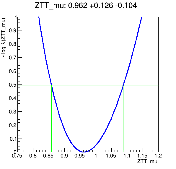
This step performs a fit on the histograms of the visible mass plot to perform a measurement.

Because the contribution of the Higgs signal is too tiny with the inclusive selection, we fit fors the “signal” strength of the Z→ττ process. You can find the fitting implementation in the Python script fit.py. Use the following command to run the fit.

mkdir -p $HOME/awesome-workshop/fit
bash fit.sh $HOME/awesome-workshop/histograms/histograms.root $HOME/awesome-workshop/fit

The resulting plot (see below) shows the scan of the profile likelihood from which we can extract the best fit value of the signal strength modifier for the Z→ττ process and the uncertainty associated with this parameter.

Key Points

• The measurement fits for the signal strength (multiplier of the Standard Model expectation) of the Z to two tau lepton process.

Final preparations

Overview

Teaching: 5 min
Exercises: 10 min

Questions

• What do I have to prepare for the workshop?

Objectives

• Run the analysis once by yourself

• Make two git repositories on CERN GitLab

• Add files to the repositories

Final preparations

We assume that you have run the analysis once by yourself and you are familiar with the different analysis steps. Follow the instructions below as final preparations for a successful workshop.

Visit GitHub/CERN GitLab and initialize the repositories

First, go to github or gitlab.cern.ch and create two new repositories using the New repository (Github) or New project (Gitlab) button. The names of the repositories should be:

• awesome-analysis-eventselection
• awesome-analysis-statistics

Check out the repositories

Next, check out the repositories. You can do this with the following command.

Github:

git clone https://github.com/<your username>/<repository name>

CERN GitLab:

git clone https://gitlab.cern.ch/<your username>/<repository name>

Add files to the repositories

Now add the files of the analysis you got from the zip archive to the repositories following the structure below. Don’t add the outputs of the analysis such as the plots and the ROOT files!

• awesome-analysis-eventselection: Files for step 1 to 3 (skimming, histograms and plots)
• awesome-analysis-statistics: Files for step 4 (fitting)

If you have never used git before, remember to set your name and email address.

git config --global user.name "<your name>"
git config --global user.email "<your email>"

Then, add the files with a meaningful commit message using the commands below.

 git add <files>
 git commit -m <commit message>

Key Points

• Run the analysis by yourself to understand the different steps.

• Set up git and visit CERN GitLab.

• Make two git repositories and add files to them.